A Comprehensive Guide to Fitting Frequency-Lowering Hearing Aids

Learning Outcomes

After this course learners will be able to:

• Describe the methods and purposes of different frequency-lowering technologies in hearing aids and evaluate their impact on speech signal processing and speech perception.
• Select and configure frequency-lowering hearing aids for different patients, considering individual audiometric profiles and technology differences, and justify their choices.
• Evaluate the outcomes associated with frequency-lowering amplification, including the limitations and potential side effects of frequency lowering, the need for individualized fitting, and the challenges and barriers in conducting research to inform evidence-based practices.

Introduction

This article delves into the advancements and methodologies in frequency-lowering technologies for hearing aids. The focus is on the technical aspects and real-world implications of these technologies. By examining different approaches and their outcomes, this article aims to provide valuable insights for audiologists and researchers, aiding in optimizing user outcomes.

Part I of this article is a big picture of the essential issues surrounding frequency lowering. Part II will review the basic steps when fitting frequency-lowering amplification. Part III provides an overview of how each manufacturer approaches frequency lowering. The remaining parts cover each manufacturer’s frequency-lowering method in detail.

Part I: Perspectives on Frequency-Lowering Amplification

Frequency Lowering is not just a ‘Feature’

Frequency lowering is not just another hearing aid feature like our other hearing aid features that provide audibility or noise reduction or those that accentuate set static signal features. Frequency lowering is different because it inserts energy into the speech signal at frequencies and times where there was none before or even where there is already energy. In this regard, frequency lowering constructively distorts the speech signal for what we hope will provide a net benefit. Frequency lowering is ubiquitous among the major hearing aid manufacturers, but it is also the least understood topic among clinicians and researchers.

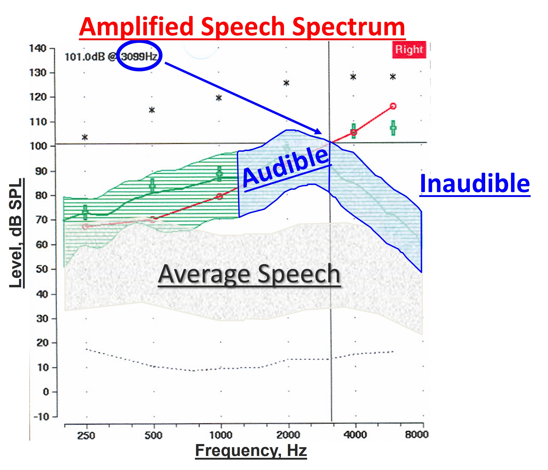
Figure 1. Probe microphone output illustrating the limitations of conventional hearing aid amplification with average speech spectrum (gray shaded area) and audiometric thresholds (red line) in dB SPL at the eardrum. The unaided speech is barely audible (below the red line). Despite amplification (green area), frequencies above 3100 Hz remain inaudible, highlighting the necessity for frequency-lowering techniques to re-code high-frequency sounds into audible lower frequencies.

Figure 1 is the output from a probe microphone and shows the fundamental problem we face with typical, conventional hearing aid amplification and the need for frequency lowering. Shown in the gray shaded area is the average speech spectrum. Everything is expressed in dB SPL at the eardrum, including the audiometric thresholds shown by the red line. It can be seen that without amplification, this particular hearing aid user is not receiving much audibility for unaided speech. The green area indicates the amplified speech spectrum and shows that despite our best efforts for this particular hearing aid user, we cannot achieve audibility much above 3100 Hz. This is where frequency lowering comes in. The idea is to take some or all of this information in the high frequencies, which is inaudible, despite our best attempts with conventional amplification, and somehow re-code it in the frequency domain. Specifically, we will take some of this information and re-code it in the lower frequencies where we can achieve audibility with our fitting.

Frequency-Lowering Information

So you might be wondering, “What is the information in the frequency-lowered signal?” Most of the representations you see depict frequency lowering in the frequency domain. This makes sense because we change the frequencies going in the hearing aid before they come out. But this is not very intuitive in terms of what the information actually is. Therefore, I propose another way of thinking about the problem in the time domain. 

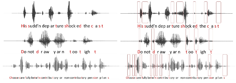
Figure 2. Comparative time waveforms of sentences with high-frequency hearing loss simulation (left) and the impact of frequency lowering (right). Inaudible phonemes for a hearing aid user are highlighted in red letters on the left. Red boxes on the right demonstrate the restoration of missing information via frequency lowering, emphasizing the enhancement in audibility and speech perception.

The left side of Figure 2 shows the time waveforms of three sentences that have been low-pass filtered to simulate high-frequency hearing loss. The letters in red are those particular phonemes that are inaudible for this particular hearing aid user. The red boxes on the right side of Figure 2 show what happens when we use frequency lowering. If you compare the left and right sides, you can see that the hearing aid user can miss a lot of information without frequency lowering. Thus, it is more apparent in the time domain that the hearing aid user now has something with frequency lowering, whereas they had nothing before.

In this respect, if we think about what information is being presented in the time domain, we have a lot of things. First, compared to when we had no frequency lowering and/or any of the acoustic signals shown here, the hearing aid user is now cued that something was said. That is, they have an awareness of the presence of sound. More specifically, they can tell from the aperiodicity of that sound that it is probably frication. And compared to other sounds that have been lowered, they have information about their duration. This might be a key feature for telling sounds apart after they have been lowered. The hearing aid user also has information about the relative intensity of the original input sound compared to others after lowering. And they have information about how that intensity changes over time, that is, the temporal envelope. You should think about these things when trying to understand the information in the frequency-lowered signal. Therefore, if you look at the time waveform, you can see it is very rich in information.

What is Lost with a Conventional Fitting?

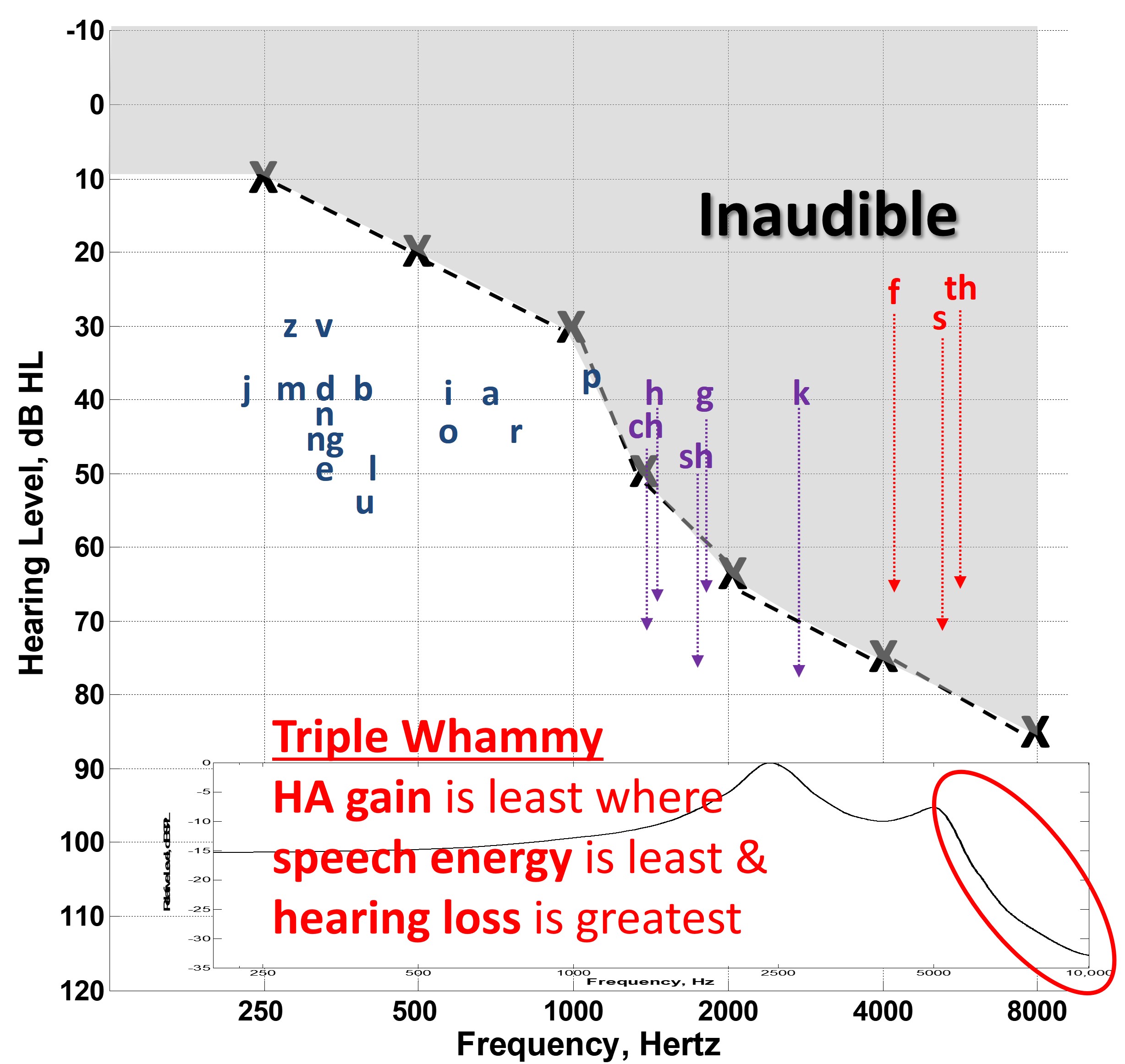
Figure 3. The ‘speech banana’ on an audiogram showing the distribution of speech sound energy by frequency and level, with low-frequency vowel energy and low-energy high-frequency fricatives (red), illustrating the difficulty in amplifying these sounds for individuals with high-frequency hearing loss (gray area). Arrows indicate the limited gain provided by conventional hearing aids for these critical sounds, especially above 5000 Hz, emphasizing the significant challenge in making high-frequency sounds audible due to minimal speech energy, significant hearing loss, and hearing aid frequency response limitations.

Figure 3 depicts the speech spectrum in a way you may be familiar with and affectionately know as the speech banana. It shows that the primary energy of importance for individual speech sounds tends to be a function of frequency and level when plotted on an audiogram. While we can appreciate that this is a gross oversimplification of speech, you can appreciate how these sounds tend to be distributed across frequency. For example, vowels tend to have more low-frequency energy. Also, the high-frequency consonants, namely the fricatives shown in red, tend to be the lowest in energy. This means that most of the energy of importance for these speech sounds is inaudible for a typical high-frequency sloping hearing loss, as shown in the gray region. We know that the primary job of hearing aids is to provide gain to make these sounds audible. However, as you see by the arrows, conventional amplification tends to be limited for these high-frequency sounds because they start with the lowest energy; therefore, they need the most gain. And because of the hearing loss configuration, they have the highest fence to clear for audibility. This is compounded by the fact that most hearing aids tend to have a frequency response that rolls off above 5000 Hz. Therefore, we have a triple whammy that conspires to make the perception of high-frequency speech difficult. Namely, that hearing aid gain is least where the speech energy is least and where the hearing loss is greatest.

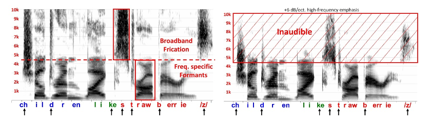
Figure 4. Left - Spectrogram of “children like strawberries” displaying the distribution of low-frequency formants (vowels, liquids, glides) versus high-frequency broadband frication (fricatives, affricates, stops). Right - The same spectrogram post typical hearing aid receiver response, highlighting the significant loss of high-frequency energy, which is not recovered even with conventional amplification, underscoring the need for frequency lowering to make fricative sounds accessible to those with high-frequency hearing loss.

The left side of Figure 4 shows a spectrogram of the sentence “children like strawberries.” Notice the overall distribution of the low-frequency sounds compared to the high-frequency sounds. In particular, notice how frequency-specific formants characterize low-frequency sounds like vowels, liquids, and glides. This differs from the speech signal in the high frequencies, which consists of broadband frication from the fricatives, affricates, and stop consonant bursts like the “k,” “t,” and “b.” The right side of Figure 4 shows the same spectrogram filtered with the typical hearing aid receiver response shown at the bottom of Figure 3. Again, notice how much energy we lose in the high frequencies. With high-frequency hearing loss, even mild to moderate hearing loss, this energy will be lost despite conventional hearing aid amplification. Therefore, the goal is to make some of this information, mainly in the fricatives, available to the user after frequency lowering.

“Just OK is not OK”

Perhaps you have seen those AT&T wireless commercials where “just OK is not OK.” Considering the potential amount of high-frequency information in the speech signal, the typical hearing aid frequency response above might be viewed as “just OK.” The thought might be that as long as you get information out to 5 or 6 kHz, you are OK because that is all you need. However, “just OK is not OK” in the context of the developmental need to access the full speech signal. A seminal study by Mary Pat Moeller and colleagues in 2007 indicated that children who were appropriately fit with conventional hearing aid amplification actually fell behind their normal-hearing peers in some of their production of the fricative and affricate sound classes. Again, “just OK is not OK.”

Clinical Barriers: Confusing Options

With the potential for frequency lowering to improve speech intelligibility and its ubiquity across major hearing aid manufacturers, you might question why it is not being utilized more in the clinic or researched more in the lab. That is, why are we still “just OK”? I think the problem lies in the fact that we have significant barriers when it comes to researching this technology and its clinical implementation. In the ideal world, evidence-based practice is where these two meet. We cannot progress until we overcome not just one of these barriers but both.

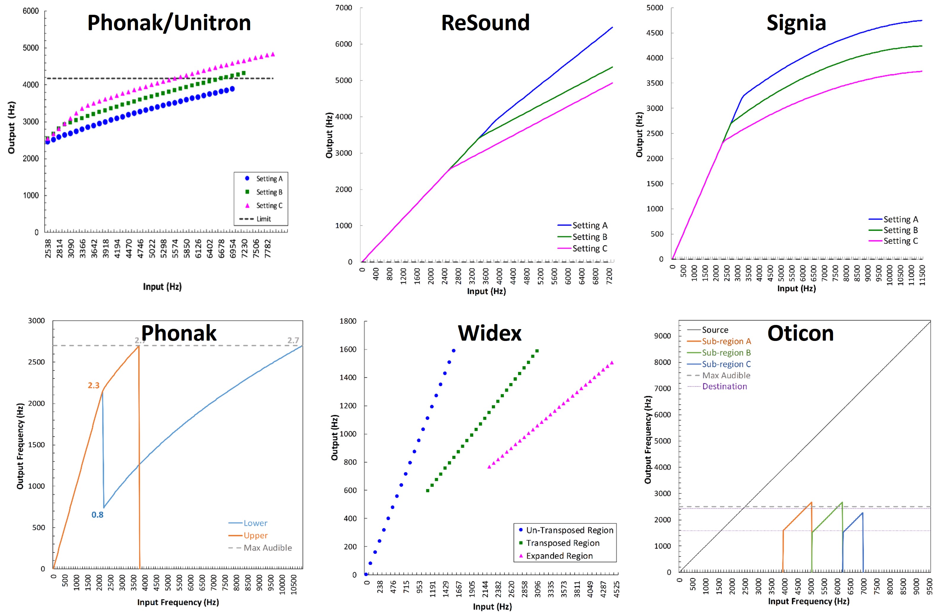
Figure 5. Panels depict examples of the frequency remapping functions used in frequency lowering by different hearing aid manufacturers, with input frequencies on the x-axis and output frequencies on the y-axis. Taken from www.tinyURL.com/FLassist, each panel represents a distinct method, illustrating both the similarities and crucial differences among manufacturers’ approaches to frequency lowering, the details of which are further examined later.

Perhaps the most significant barrier to the clinical implementation of frequency lowering is the variety of options each manufacturer offers. It is unclear what is happening underneath the hood regarding the information provided by the different manufacturers. Each panel in Figure 5 shows a different frequency-lowering method using frequency remapping functions. These functions show frequencies going into the hearing aid along the x-axis and frequencies going out along the y-axis. While some of them look similar, they differ in significant ways discussed in detail later.

When it comes to research, we have conceptual and technological barriers. Of course, we know the number one thing you need for good quality research is double-blinded randomized control trials. A related reason is that there is limited access to control the technology and/or an understanding of what the hearing aids are doing to conduct the proper experiments in the first place. The idea is that you know if you are confined to just what you can do in the programming software, and if those options vary depending upon the audiogram you enter for your hearing aid user, it is difficult to do the proper control study. To a considerable extent, related to what is happening clinically, researchers do not have a solid understanding of the technology — and it is not their fault. The fact is that there is a limited amount of information provided by the manufacturers about what is really happening. This information is critical in order to carry out the proper experiments.

Research Barriers: Conceptual & Technological

We also have limited individualization within the research realm. Again, this is related to the lack of control and understanding of the technology. What happens in many of these studies is that the subjects are fit with the same settings. One of the things that I want to emphasize here is that you have to individualize the settings for your hearing aid user and the amount of audibility you have to work with. The other thing you see is that researchers simply use the manufacturer’s idea of what is right based on the audiogram, not aided audibility. As a result, the fitting is not individualized how it needs to be. This is equivalent to just giving everybody the same gain settings. If we give everybody the same gain as a function of frequency, you can expect it will be too much for some people. For other people, it is going to be too little. Therefore, when you look at outcomes across the board, you should not be surprised when you do not have conclusive results regarding whether it works.

Guarantees with Frequency Lowering

With all this being said, how does it translate into the outcomes expected with frequency lowering? First, let me summarize by explaining the guarantees associated with fitting frequency-lowering hearing aids. Give me a hearing aid with frequency lowering, and I can guarantee you that I can make speech understanding worse, a lot worse. Later, I will explain why and what you must be aware of when using this technology. I can almost guarantee you that I can preserve speech understanding. That is, “do no harm” if it is fit appropriately. I cannot guarantee you that I can always make speech understanding better.

Potential Side Effects

Regarding the potential side effects, we must remember that while the speech code is relatively scale-invariant, we can turn it up and down. Doing so will not change the identity of sounds because, as we know, it is heavily dependent on frequency. While I do not necessarily view frequency-lowering as a feature, no other hearing aid feature has as much potential to change the identity of individual speech sounds. Therefore, it can worsen speech understanding because the low-frequency information has to be altered somehow to accommodate the displaced high-frequency information. Said another way, the re-coded information from the high frequencies has to go to frequency regions that we would otherwise choose to fit normally with conventional amplification. Therefore, we intentionally alter the speech signal using constructive distortion — hopefully, for an overall net gain. The concern is not so much the fidelity of the recorded information, that is, how much it mimics or matches the existing high-frequency information. Instead, we must be concerned about how the newly introduced distortion and overall sound quality might work against us.

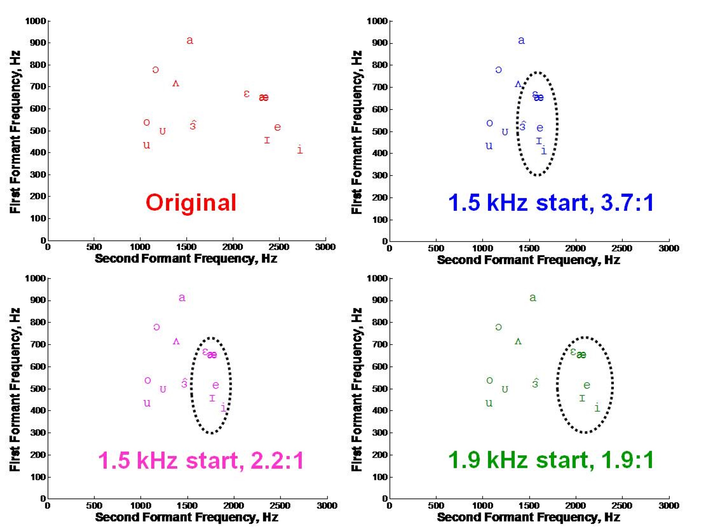
Figure 6. Vowel space representation with the first formant on the Y-axis and the second formant on the X-axis. The upper-left panel (in red) shows the standard vowel space, while subsequent panels demonstrate the effects of nonlinear frequency compression at various ratios, indicating the potential alteration of vowel identity due to the squeezing of formants, with higher ratios resulting in greater compression and potential confusion of vowel sounds.

As indicated earlier, most of the information in the low-frequency speech spectrum is frequency-specific. Specifically, we have formants with consonants like liquids and glides. We also have formants in the vowels. These formants transition into and out of the different consonants. Recall from basic speech acoustics that you can categorize our vowels acoustically according to their first and second formant frequencies. As shown in Figure 6, the first formant is on the Y-axis, and the second formant is on the X-axis. This is typically called the vowel space. The upper-left panel in red is the typical unaltered vowel space. With nonlinear frequency compression, which I detail later, the information above the start frequency is squeezed down by different ratios. Higher ratios result in more squeezing. We know that vowel identification is tightly tied to where the formants are, so we might change the vowel identity if we change the formants. And the closer the formants are, the more they will be confused.

Balancing the Positives Against the Negatives

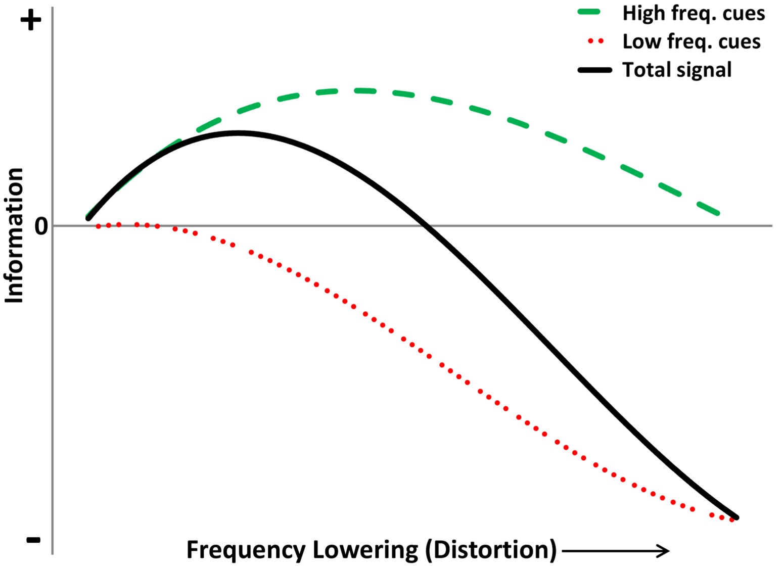
Figure 7. Hypothetical model correlating information (y-axis) with the degree of frequency lowering/distortion (x-axis). The green dotted line represents high-frequency information gain, which increases with frequency lowering to an optimal point before it diminishes due to acoustic overlap. The red line shows how low-frequency information is preserved or distorted by frequency lowering. The black line, the sum of green and red, illustrates the non-monotonic total information trajectory, peaking before decreasing as speech understanding worsens, emphasizing the balance needed in frequency lowering to enhance overall speech comprehension.

All of this can be summarized with the following hypothetical model. Shown along the y-axis is a metric of information, and along the x-axis is the amount of frequency lowering, which is synonymous with distortion. Recall that frequency lowering if done right, will be constructive distortion. What we want to avoid is destructive distortion. As shown by the green dotted line, as the amount of frequency lowering increases, so does the amount of information from the high frequencies, but only up to a point when the informational value decreases. It does this because the lowered signals overlap more and more so that the high-frequency sounds are no longer distinguishable — they sound the same. Considering the other side of the spectrum, the red line indicates that mild or moderate frequency lowering can preserve information from the low frequencies with most techniques. However, as shown in Figure 6, you can overdo it: if you keep increasing the degree of frequency lowering, you will increase the distortion of the low-frequency information. The total information, the black line, is the sum of the green and the red lines. The predicted relationship is non-monotonic such that it reaches a peak, then it becomes negative at some point such that overall speech understanding worsens. The point at which this occurs likely depends on the interaction with other factors like the individual hearing loss and the specific frequency-lowering technique. The critical teaching points are that less can be more and that a successful fitting will give the listener more than what is taken away.

To Fit or Not to Fit, that is the Question

Ultimately, a decision has to be made whether or not the potential pros outweigh the cons. If the hearing aid user experiences speech perception deficits with conventional amplification despite your best efforts to achieve high-frequency audibility, it might be a deciding factor. If the decision is to fit, there are a few things that you need to ask. First, “how does the technology of choice work?” The manufacturers have fundamental differences regarding the techniques, terminology, and what happens when you adjust the settings. Refer back to Figure 5, showing all the differences between the manufacturers. Second, you must know what is happening underneath the hood to make an efficacious decision for your hearing aid user. Third, you must also know how much of the lowered information is audible. This will be the topic of Part II. And then, finally, you must ask, “Can the hearing aid user use the lowered information?” Your validation measures will answer this, whether they consist of a speech test, a pencil and paper questionnaire, or simply open-ended questions.

Part II: Using Probe Microphone Measures to Optimize Outcomes with Frequency Lowering

The Importance of Probe Microphone Measures: Making Sure the Cure is Not Worse than the Disease

One of the takeaway points from Part I was the importance of minimizing potential side effects associated with frequency lowering. To facilitate this goal, knowing what to look for when doing probe microphone measurements is essential. You know the importance of doing probe microphone measures for conventional amplification, which does not change for hearing aids with frequency lowering. However, when using frequency lowering, you want to look for additional things in the amplified spectrum. Therefore, with the possibility of side effects causing harm by altering low frequencies or implementing too much frequency lowering, you must know what you are delivering to the hearing aid user. Part of this has to do with knowing what the output is. Probe microphone measures will tell you the hearing aid output after frequency lowering. You might know what the input is, but you will not know the relationship between input and output. The relationship between input and output for each manufacturer will be discussed later. While probe microphone measures will not tell you this relationship, there are things you want to look at for the output.

It is common for individuals to stop taking a medicine because they prefer the original disease to the side effects. Let us think about this in the context of a hearing aid with frequency lowering. If you fit it inappropriately — to the point where they have side effects — they may not understand speech as well. Therefore, they may go without hearing aids, return the product, and never see you again.

Primary Goals for Probe Microphone Measures

There are specific things you want to do for each manufacturer and how they approach frequency lowering. However, there are some commonalities when doing probe microphone measurements. Three key goals transcend all of the different techniques.

1. The audible bandwidth after frequency lowering is activated should not be less than before. The critical thing is that you do not want to reduce the audible bandwidth. If you can achieve audibility up to a particular frequency, you want to use that real estate as much as possible. You want to avoid using so much frequency lowering that it takes away from what you had to begin with because you are working against yourself. Think about this in the context of overall net benefit: you want to provide additional high-frequency information while maintaining or minimizing detriment to the existing low-frequency information.
2. The lowered information should be audible. This seems obvious, but it is not because, depending upon the technology, you cannot always tell that the lowered information is audible by looking at the output. How can you know what went into the input when all you have is the output? Manufacturers define things slightly differently and operate in different ways, so it is possible to get confused. It is not uncommon for all frequency lowering to happen at a range where the hearing aid user has no audibility, especially if you use the manufacturer’s default settings. In this case, you should not be surprised that the hearing aid user reports no benefit. Remember Part I, where it discussed the clinical and research barriers? It is the same situation on the research side of things. If everybody is fit with the same setting using a manufacturer’s default, then you really have no control over how much of the lowered information is put into a range of audibility. I have developed online tools to help address this goal; these will be discussed later.
3. Use the weakest frequency-lowering setting to accomplish your objective. This objective may vary depending on the severity of hearing loss. For example, you might do slightly different things if you are fitting a mild-to-moderate hearing loss versus a moderately-severe hearing loss. How do you know which setting is the weakest, and how do you know you are accomplishing your objective? Again, this is where my online tools come into play.

A Protocol for Fitting Frequency-Lowering Hearing Aids

While the methods used for frequency lowering differ across manufacturers, we can establish a generic protocol for fitting all frequency-lowering hearing aids.

1. Deactivate the frequency lowering and then fit the hearing aid to prescriptive targets with the DSL, NAL-NL2, etc., using probe microphone measures just as you would for a conventional hearing aid. The point is to see how much you can reach the targets.
2. With the frequency lowering still deactivated, find the maximum audible output frequency (MAOF). The maximum audible output frequency is the highest frequency at which the aided output exceeds the threshold on the SPL-o-gram. The objective is to determine how much real estate you have to work with.
3. Activate frequency lowering and use the online tools to position the lowered speech into the audible bandwidth, that is, below the MAOF. While you want to fit the lowered speech in that region, you do not want to reduce what you had to work with before. The destination region is where the frequency-lowered information will be at the output, so most of the lowered speech must be below the MAOF to be audible. At the same time, you want to avoid too much lowering, which can introduce side effects to the point where you have zero or negative overall net benefit, thereby compromising speech intelligibility.
4. Once you have selected the setting that matches the overarching goals highlighted earlier, the last thing to do is re-run the speechmap and ensure that the MAOF is reasonably close to what it was when frequency lowering was deactivated.

The Maximum Audible Output Frequency (MAOF)

Going back through my records, the term “maximum audible output frequency,” affectionately known as the MAOF, was born on March 30, 2009. Referring to Figure 1, when you look at the aided speech spectrum shown by the green-shaded area, the maximum audible output frequency tells you how much real estate you have to work with before frequency-lowering is activated. As shown by the arrow pointing to 3100 Hz, the MAOF is somewhere between the frequencies at which average speech and the peaks of speech cross the line (red in this example) corresponding to the threshold. You must use your judgment about where you choose along this line, but in this example, I chose where the peaks of speech cross the threshold line. The MAOF tells you at least two things. First, it tells you the severity of the deficit — that is, how much sound the hearing aid user is missing or how much of the speech spectrum is inaudible. Second, it gives you an idea of how much real estate you have to work with or the range of audible frequencies available for re-coding some of the inaudible high-frequency speech information. Of course, the lower the MAOF is, the more deficit you have and the less room you have to work with when trying to re-code it.

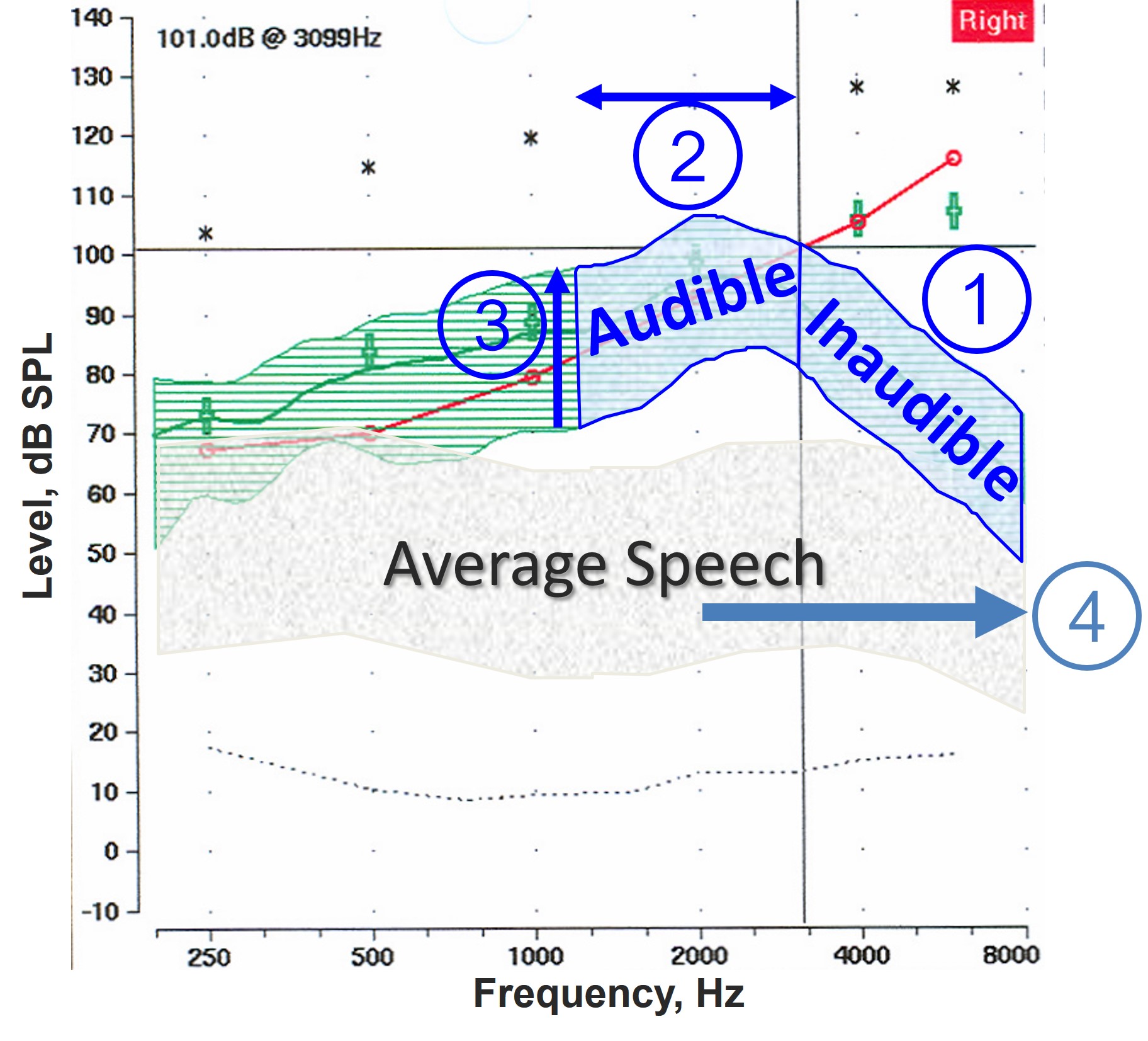
Figure 8. Probe microphone output illustrating the challenges of enhancing audibility while preserving speech information integrity with frequency-lowering techniques, including (1) potential distortion or truncation of the inaudible information, (2) possible masking of existing sounds when repositioning the information, (3) the necessity of amplifying the newly coded signal in areas of cochlear damage, and (4) the inherent deficit created by limited bandwidth in the average speech spectrum, summarizing.

As indicated by Figure 8, the overall net benefit from frequency lowering is limited by at least four things.

1. When you have a region of inaudibility, the particular method may have to distort this information. That is, you might have to squeeze it using compression and/or you might have to truncate it by taking only a limited part of the total inaudibility range instead of the full bandwidth. So, you may not be moving all the information in the original input signal.
2. When you move the missing information, you must put it where the hearing aid user can hear it. Sometimes, there may be coexisting sounds at the same time at those particular frequencies so you run the potential of masking the information already there. Or, to accommodate the new frequency-lowered information with compression techniques, you may have to move information in the audible region that would be amplified normally through the hearing aid.
3. As indicated by the up arrow, you must amplify the frequency-lowered signal. The significance of this is that newly re-coded information must be put on the cochlea where there is probably some existing outer and inner hair cell damage.
4. As indicated by the rightward-facing arrow in the average speech spectrum (gray-shaded area), the size of the deficit may limit the benefit from frequency-lowering. In other words, the amount of information lost when bandwidth is reduced for normal-hearing listeners. So, in this sense #4 establishes the size of the deficit, that is, the net loss of information due to limited bandwidth and #1, #2, and #3 influence how much this deficit can be recovered with frequency-lowering. 

This is just a laundry list of things that limit the total benefit you may get compared to simply extending bandwidth. In summary, you may need to put a limited amount of information from the inaudible region in a region with low-frequency speech information and sensorineural hearing loss.

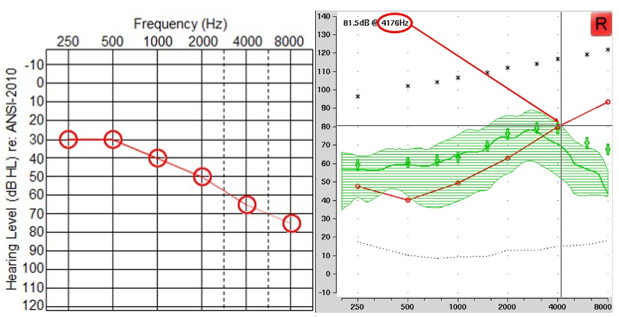
Figure 9. Left panel displays an example audiogram, while the right panel shows the SPL-o-gram of the aided speech spectrum. The maximum audible output frequency is marked by a red arrow at 4176 Hz, indicating the highest frequency at which audibility is achieved.

I go through two example audiograms for each manufacturer. Figure 9 shows the first example. The audiogram is shown on the left, and the SPL-o-gram of the aided speech spectrum is shown on the right. Again, the maximum audible output frequency is the highest frequency at which we have audibility. In this case, it is 4176 Hz, as indicated by the red arrow. Some people have argued that you should use the average. I have always used the peak since the frequency where the aided speech spectrum crosses audibility can vary depending on vocal effort and environmental acoustics. Furthermore, the peaks of some high-frequency sounds like “s” and “sh” contain speech information that can be useful, so I have always used the peak, but I also tell people to use their best judgment. For example, if we instead had only a sliver of barely audible information extending over a range of 1000 or 2000 Hz, then using your judgment, you would say there is no way that a person can use that information. So again, it does not have to be an absolute thing, but this is a nice, clean case.

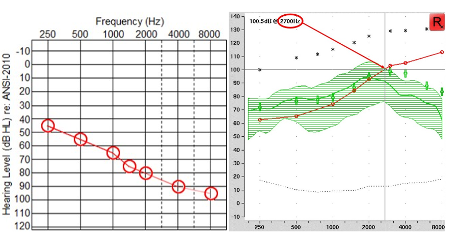
Figure 10. Left panel displays an audiogram with more significant hearing loss than the example in Figure 9. The right panel shows the SPL-o-gram of the aided speech spectrum and the maximum audible output frequency at 2700 Hz.

Figure 10 shows the second example that will be used in later. Again, using the frequency where the peak of the aided speech spectrum crosses the line of audibility, the maximum audible output frequency for this example is 2700 Hz.

Using the MOAF and the Frequency-Lowering Fitting Assistants

The information obtained from the probe microphone measures, namely, the maximum audible output frequency, can be used in conjunction with my frequency-lowering fitting assistants, which will be the focus of the latter parts of this article. I have developed these tools for each major hearing aid manufacturer to show you how frequency is allocated with their different frequency-lowering settings. So, even if you do not buy into the goals I establish for each manufacturer, demystifying what is going on with the individual technology can effectively reduce the clinical barriers I discussed earlier.

The purpose of the frequency-lowering fitting assistants is not necessarily to determine optimal settings but rather to empower the clinician. They can do this by providing information about how sounds are changed with the different settings. Then, they can help you reduce all the available settings into a reasonable set based on first principles. These are our guiding principles for making different parameter selections. For example, the primary first principle is to maintain the audible bandwidth available before frequency lowering was activated. The other first principles will vary depending on the technology reviewed in Part III.

Recall the research and clinical barriers discussed in Part I, manifesting as a lack of control and standardized methodology. Therefore, if nothing else, they can set a benchmark to promote uniformity across clinicians, protocols, test sites, or whatever else. The idea is that, as a field, we can establish some agreed-upon way of fitting this technology, and once we do this, we can start to examine whether or not there is any other, maybe different, set of principles that we should be using. But we have to start somewhere.

What Acoustic Feature(s) Should We Optimize for Best Outcomes?

With what has been said so far, we must stop and question what should be optimized when looking at the output from probe microphone measures. At some point, we need to question what is meant by “optimization.” These questions have important implications for algorithm design. They also have important implications for selecting a particular method of frequency lowering and adjusting its parameters for individual hearing aid users.

While there is no firm conclusion, conventional wisdom adheres to an untested assumption that the spectral features of the high-frequency cues need to be preserved or replicated in the lowered signal. This has led to two common recommendations for optimizing fittings. The first one is in terms of the input bandwidth. That is, how much of the input signal can we actually lower? The problem with that is that more is not always better. For example, suppose you have two frequency-lowering settings, one of which can lower input frequencies up to 9000 Hz and the other up to only 7000 Hz. Under this premise, the setting that puts sounds up to 9000 Hz into the region of audibility would be more optimal than the one that puts sounds only up to 7000 Hz. However, as I highlighted in Part I, too much frequency lowering can harm speech intelligibility. So, while one setting might make more information from the input audible, the usability of that information might not be as good. The second recommendation that falls out of the notion that optimization should occur in the frequency domain involves the “s” and “sh” sounds because they constitute the biggest source of confusion with frequency lowering. The idea is to keep these key sound contrasts as separate as possible in the output after lowering. An example of this will be illustrated at the end of Part II.

Other, Less Precise Methods using Probe Microphone Measures

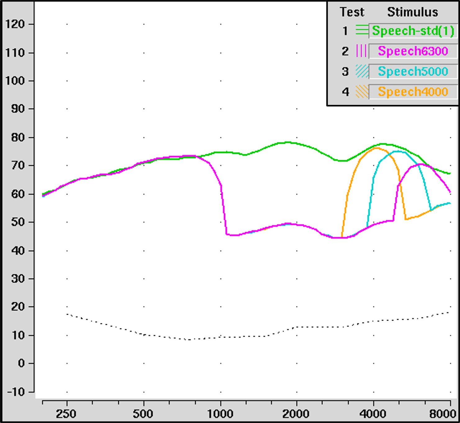
Figure 11. The input spectrum for the standard speech stimulus in the Audioscan Verifit is shown in green. The special speech signals with high-frequency energy centered at 6300, 5000, and 4000 Hz are shown in magenta, blue, and yellow, respectively. Not shown is the special speech signal centered at 3150 Hz.

A few years after the first modern hearing aids with frequency lowering were introduced, Audioscan created special speech signals to help clinicians visualize frequency lowering in action. These are available from the selection menu containing the rest of the input signals. Essentially, they reduced most of the energy in the standard speech signal above 1000 Hz except for a 1/3-octave band centered at 3150, 4000, 5000, or 6300 Hz. As I discussed earlier, you do not know the input-to-output frequency mapping since you can only see the output. The purpose of these signals is to constrain the input to make it easy to visualize where it goes in the output.

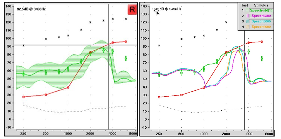
Figure 12. After frequency lowering, the left panel depicts the aided speechmap for the standard speech signal, without a clear indication of the input. The right panel displays the output of the special speech signals: the magenta line represents the 6300 Hz input remapped to 3200 Hz; the blue line shows the 5000 Hz input shifted to around 2500 Hz; and the yellow line indicates the 4000 Hz signal shifted to around 2000 Hz. The visibility of these lines relative to the threshold line (red) offers insights into the audibility of specific input frequencies, with some important caveats.

The left panel of Figure 12 shows the aided speechmap for the standard speech signal with frequency lowering activated. It is not apparent which parts have been lowered and from whence they originated just by looking at it. The right panel shows the output for each of the three special speech signals shown in Figure 11. The magenta line is for the speech signal that originated at 6300 Hz. Notice that it shows up around 3200 Hz with frequency lowering. Similarly, the blue line for the 5000-Hz special speech signal shows up in the output at around 2500 Hz, and the yellow line for the 4000-Hz signal shows up at around 2000 Hz. One idea is to use these signals to determine how much audibility you have from the original input signal. For example, for the 6300-Hz signal, you can see that it is below audibility, while the 5000-Hz signal is just barely audible because it is slightly above the threshold line. Interestingly, notice that the 4000-Hz signal does not appear to be audible. I explain why this might be in the following paragraphs.

While Figure 12 demonstrates the utility of the special speech in providing some gross information about where you lose audibility for the lowered input signal, it is an incomplete picture of the entire frequency remapping function. Furthermore, there are other problems I have identified with them. First, recall that they are only 1/3-octave wide at the input to the hearing aid. Also, note that the analysis bands are only 1/3-octave wide. The problem is that frequency compression (discussed in Part III) will squeeze the input signal so that its output is narrower than 1/3 octave. Because actual running speech has high-frequency energy wider than 1/3 octave, the special speech signals may lead you to underestimate the actual output from the hearing aid when frequency compression is engaged.

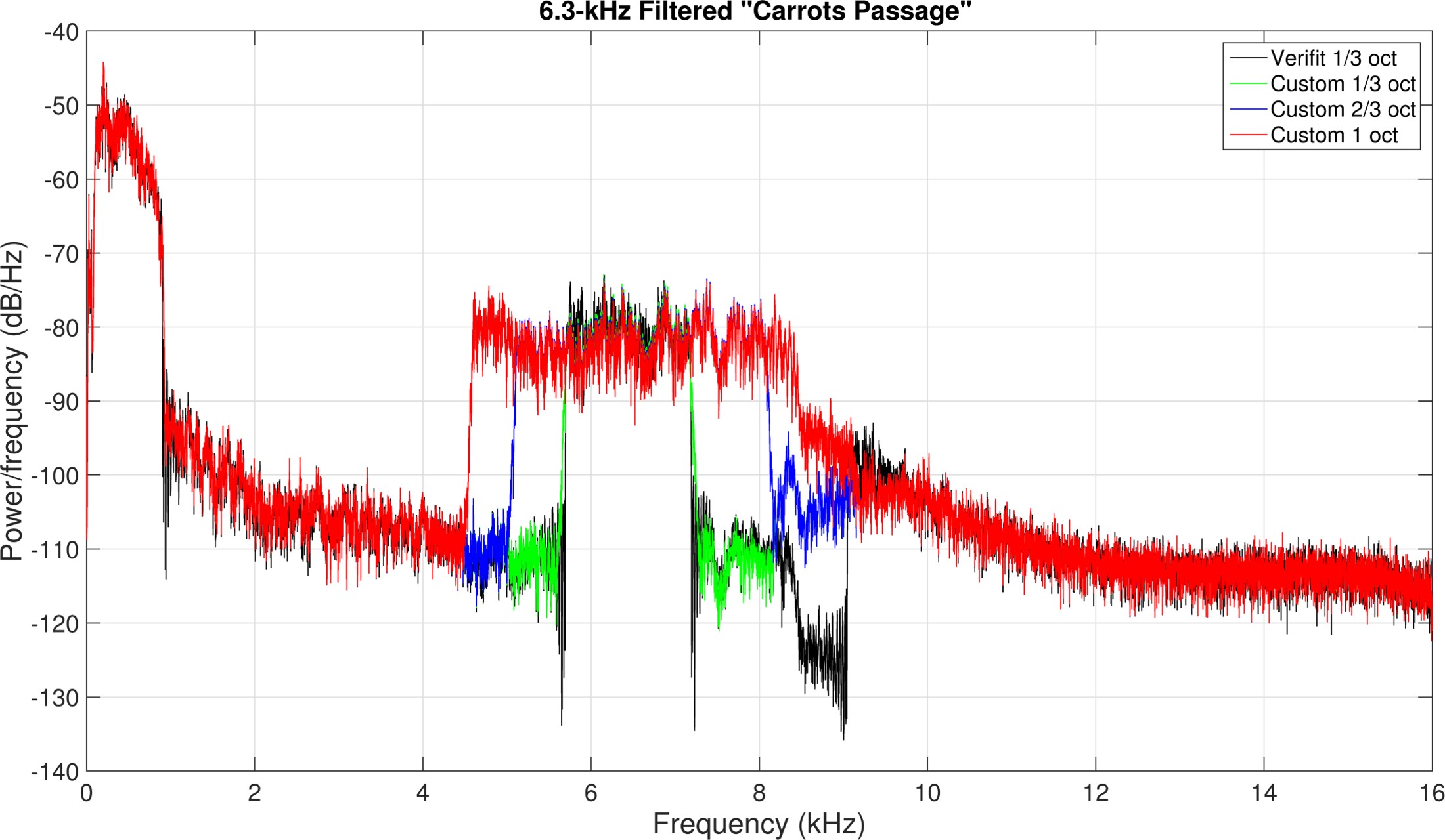
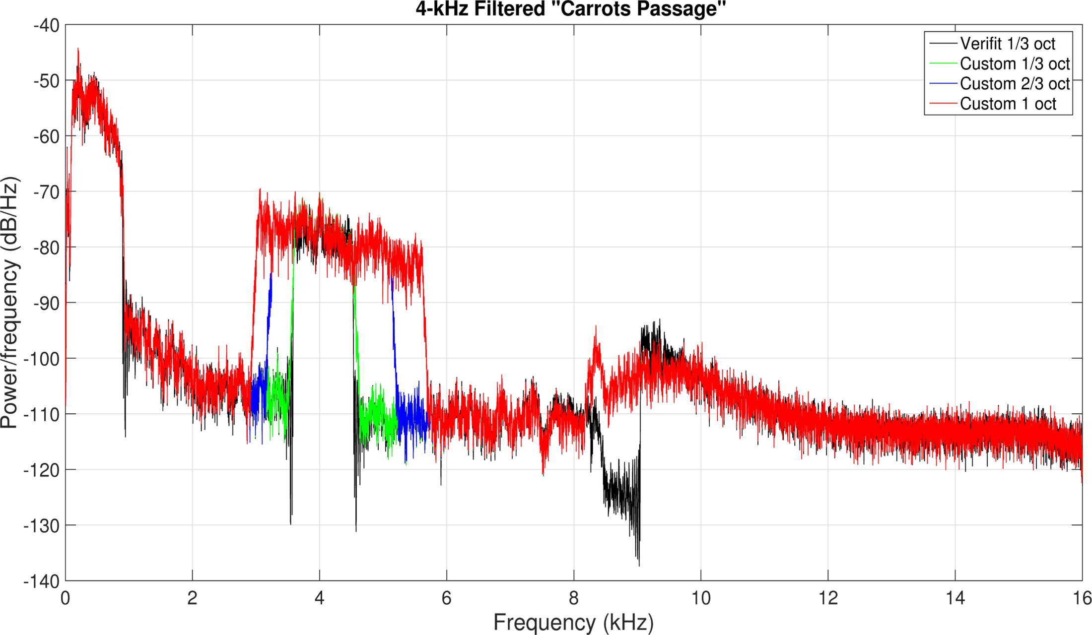
Figure 13. The top panel displays spectra of signals centered at 6300 Hz. The bottom panel shows spectra of signals centered at 4000 Hz, created to highlight issues with using the special speech signals in hearing aids using frequency compression. The original special speech signals from the Verifit are depicted in black, while the green signals represent those recreated for method validation. The blue and red signals illustrate the effects of different filter widths, 2/3-octave, and 1-octave, respectively.

Figure 13 shows signals I created to demonstrate the problem faced when using the special speech signals on hearing aids with frequency compression. I used the standard carrot passage from the Verifit and filtered it with three different filters. The top panel shows the spectra of the signals centered at 6300 Hz, and the bottom panel shows the spectra of the signals centered at 4000 Hz. The original special speech signals from the Verifit are in black, and the ones I created to check my methods are in green. The 2/3-octave wide signals are in blue, and 1-octave wide signals are in red.

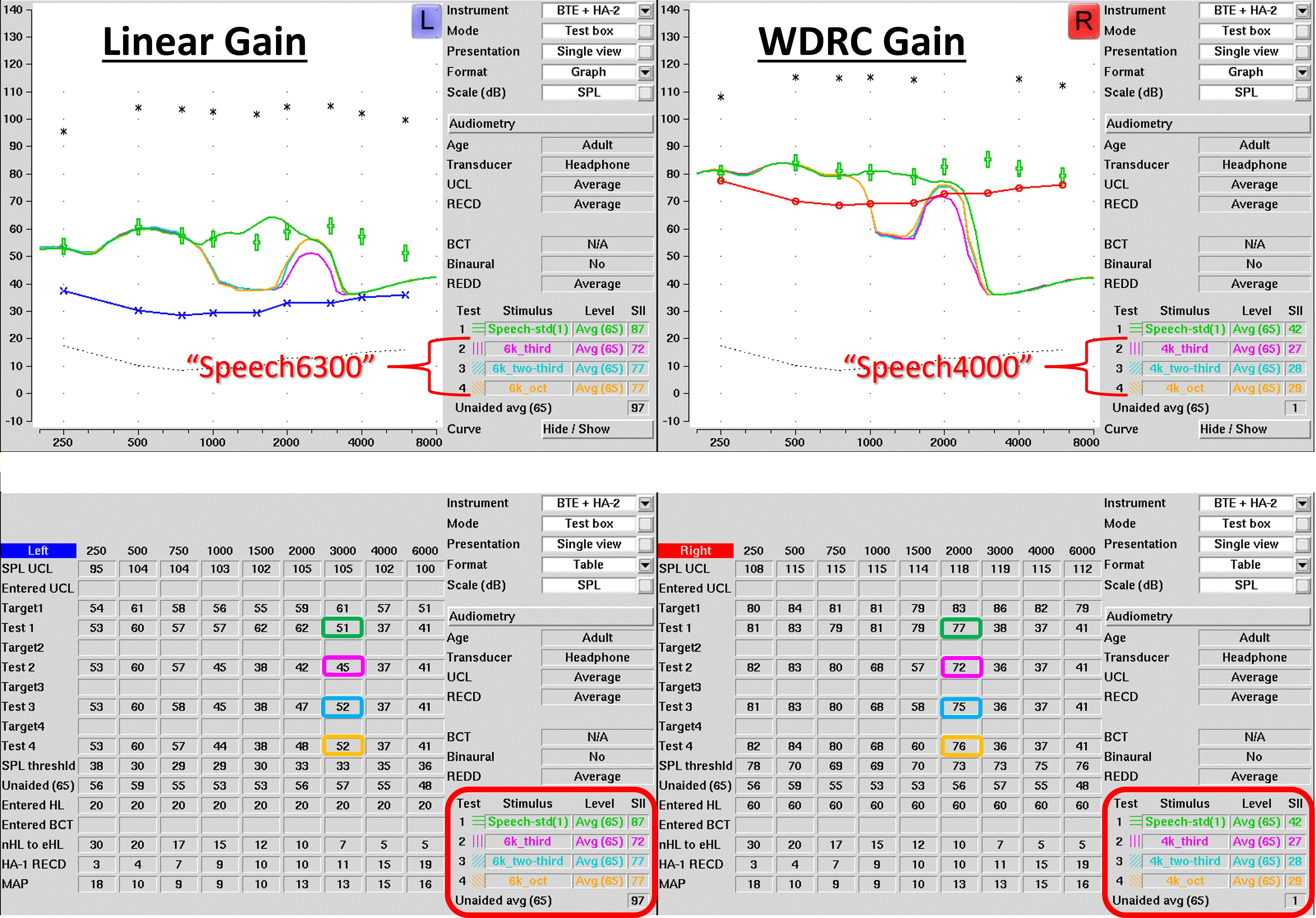
Figure 14. Speechmaps of signals (from Figure 13) processed by a hearing aid with frequency compression. The left example uses linear gain, displaying green (standard speech signal), magenta (1/3-octave wide signal at 6300 Hz), blue (2/3-octave wide), and gold (1-octave wide) lines, with all special signals appearing around 3000 Hz in output. Notably, the magenta line is lower than others, as quantified in the accompanying table. The right example demonstrates a hearing aid with WDRC gain, showing a smaller error for the magenta special speech signal because WDRC provides more gain for lower input levels.

Figure 14 shows the speechmaps for the signals shown in Figure 13 when processed with a hearing aid using frequency compression. The example on the left is for a hearing aid with linear gain. Just as before, the green line corresponds to the standard speech signal. The magenta line corresponds to the 1/3-octave wide speech signal centered at 6300 Hz. The 2/3-octave wide and 1-octave wide signals are shown in blue and gold, respectively. Notice that each special speech signal originating from 6300 Hz appears in the output around 3000 Hz. Also, notice that the magenta line, equivalent to the Verifit special speech signal, is lower than the others. The differences can be quantified using the numbers in the table. Notice for the standard speech signal (Test 1), the analysis band centered at 3000 Hz is 51 dB. Meanwhile, the output for the 1/3-octave wide input signal is 45 dB (Test 2), which is 7 dB less than the output for the wider signals, whose output levels are about the same as for the standard speech signal. Again, this happens because the output bandwidth of a signal 1/3-octave wide at the input will be less than 1/3-octave wide when compressed in frequency. On the other hand, the other two signals in Test 3 and Test 4 fill the full analysis band after frequency compression, so their output levels are higher. The example on the right is for a hearing aid with WDRC gain. For this example, there is still an error associated with the special speech signal in magenta, but it is smaller because lower input levels receive more gain.

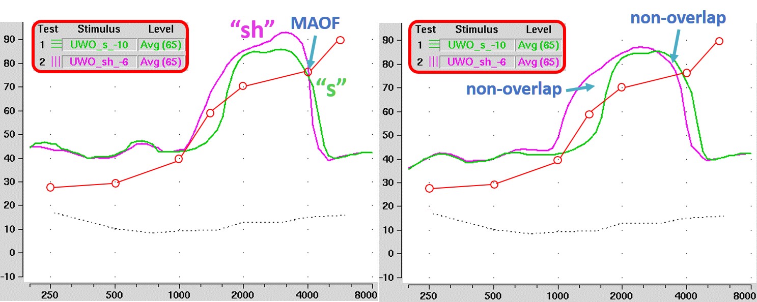
Figure 15. Illustration of the process for utilizing the calibrated “s” and “sh” sounds in the Verifit. Step 1 involves determining the Maximum Audible Output Frequency (MAOF) without frequency lowering. Step 2 (left) checks the audibility of these sounds by comparing their speechmaps (with “s” shown in green) against the threshold line, aiming for the “s” output to align approximately with the MAOF. Step 3 (right) involves selecting settings that minimize the overlap between the “s” and “sh” sounds, assuming that this will optimize the clarity and distinctiveness of these sounds with frequency lowering activated.

The second set of signals in the Verifit designed for frequency-lowering hearing aids falls out of the notion that optimization should occur in the frequency domain. In particular, these are calibrated “s” and “sh” sounds because, as indicated earlier, this is the biggest source of confusion with frequency lowering. The calibrated “sh” has energy up to 6000 Hz, and the “s” has up to 10,000 Hz. The goal is to keep these key speech contrasts as separate as possible after lowering.

Figure 15 demonstrates the procedure for using these special signals. After obtaining the MAOF with frequency lowering deactivated (step 1), step 2, as shown on the left, is to ensure the two sounds are audible by comparing their speechmaps to the threshold line. Ideally, the upper edge of the output for “s” (green line) will approximate the MAOF. The purpose is to ensure that all or most of the lowered sounds are audible. After you have found the settings that make “s” audible, step 3, as shown on the right, is to choose the setting that has the least amount of overlap between the “s” and “sh.” My only problem with this metric is that according to my research, the separation between these two sounds after lowering is often not big enough to be perceptible even to people with normal hearing. In other words, you must make the frequency differences between these sounds relatively large to notice them.

Part III: Overview of Frequency-Lowering Techniques

The purpose of Part III is to provide a broad overview of the different techniques by which manufacturers today achieve frequency lowering. Subsequent parts will focus on each manufacturer in greater detail.

Frequency Lowering Techniques by Manufacturer

Frequency lowering is ubiquitous; each major manufacturer offers some version of frequency lowering. However, it is also the most misunderstood feature of hearing aids today. The remainder of this article aims to clarify some of this misunderstanding. 

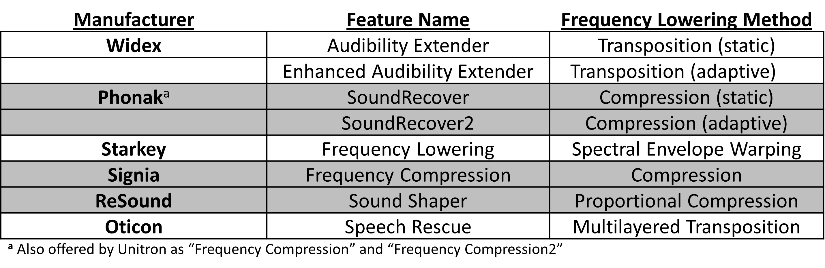
Table I. A categorization of the major hearing aid manufacturers by their frequency-lowering feature, listing them in chronological order of release (first column). The second column provides the specific names of these features. The table also distinguishes the frequency-lowering techniques used — color-coded as transposition (white rows) and compression methods (gray rows), with the specific method listed in the third column.

Table I provides a comprehensive overview of the frequency-lowering techniques utilized in modern hearing aids. The first column lists the names of hearing aid manufacturers in the order of the historical release of their frequency-lowering features, beginning with Widex and concluding with Oticon. This chronological listing provides a historical perspective on the evolution and adoption of frequency-lowering technology. The second column lists the specific names assigned by each manufacturer to their frequency-lowering technology. It also notes subsidiaries and associated brands that offer similar technologies using different terminology. The final column describes the specific technical approach employed in the frequency-lowering process. Further details on these techniques are provided in the subsequent parts of the article. The rows of the table are also color-coded: white rows denote transposition techniques, and gray rows indicate compression techniques.

Terminology Review

It will be helpful to review some terminology before getting into specifics. The source region refers to the frequency range from which information is being moved. It refers to the frequencies that are being moved down lower. Depending upon the manufacturer, the lowest frequency in this source region is the “start,” “cutoff,” or “f_min” for the minimum frequency. The target or destination region is the frequency range where information from the source region is moved to. Depending on your source of information, there is some confusion between and between frequency compression and frequency transposition, which are often used interchangeably. However, the terms refer to particular techniques that should not be confused.

Frequency Compression

Imagine frequency compression like an uncoiled spring divided into two sections, divided by a “start” frequency. The first half is uncompressed, while the second half is squeezed. If the length of the spring represents frequency, frequency compression progressively moves the higher frequencies down so that they end up being squeezed, and the differences between them become closer. The target region (the squeezed high-frequency section) is contained within the source region (the uncoiled high-frequency section), with the target region being pushed toward the start frequency; thus, the output bandwidth is reduced. Part II emphasized the importance of maintaining the audible output bandwidth after frequency lowering so that it is at least as large as before frequency lowering.

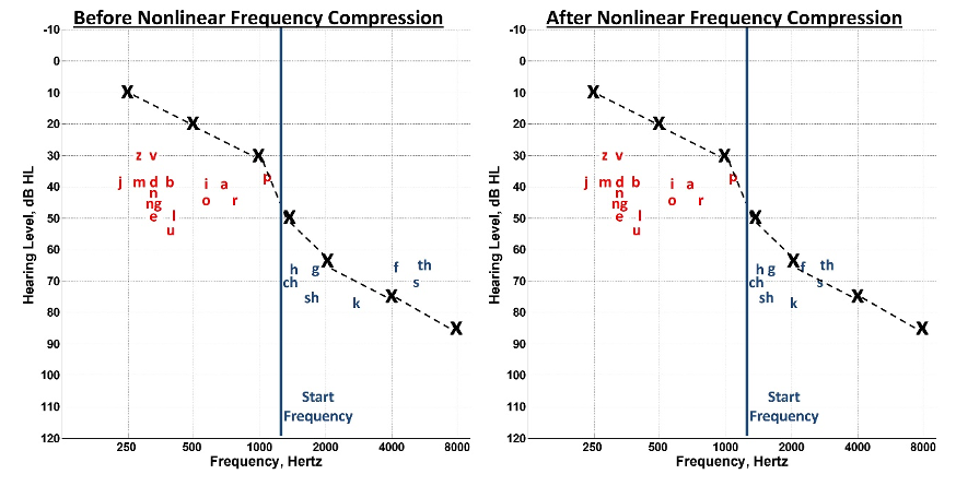
Figure 16. Comparison of speech information before (left) and after (right) nonlinear frequency compression. The frequency range is divided at a start frequency (blue line), with sounds below this point (in red) remaining unchanged, while sounds above it (in blue) are shifted downwards to enhance audibility through the hearing aid.

Part I reviewed how low-intensity, high-frequency sounds, namely the fricatives, are still inaudible despite our best attempts to amplify speech (see Figure 3). Figure 16 represents the speech information shown in Figure 3 before (left) and after (right) nonlinear frequency compression. The basic idea is to divide the frequency range into two parts at a given start frequency, as represented by the blue line. The sounds below the start frequency, shown in red, are unaltered. The sounds above the start frequency, shown in blue, are moved down into a region where audibility with the hearing aid can be achieved.

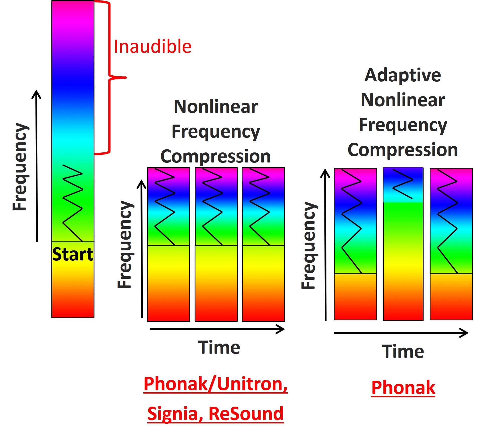
Figure 17. Schematic of the nonlinear frequency compression approaches in hearing aids. The color bar on the left indicates incoming frequencies, with low frequencies in red at the bottom and high frequencies in magenta at the top. The figure illustrates the division of the spectrum at a start frequency, where frequencies above are lowered. Middle of the figure shows the basic technique used by Phonak, Unitron, Signia, and ReSound, highlighting their nonlinear frequency compression method. The right side depicts Phonak’s latest approach, adaptive nonlinear frequency compression, which employs two cutoff frequencies to adaptively alter high-frequency sounds, like fricatives, and preserve low-frequency sounds, like vowels and harmonics, enhancing audibility without significantly altering the sound quality.

Figure 17 is a schematic of the different frequency compression approaches. The color bar on the left represents the frequencies going into the hearing aid. The low frequencies are toward the bottom in red, and the high frequencies are toward the top in magenta. Assume that the upper half of the frequency range is inaudible despite our best attempts to achieve audibility with the hearing aid. One of the characteristics of nonlinear frequency compression is that it divides the incoming spectrum into two parts as designated by the start frequency. Everything above the start frequency is then subjected to frequency lowering. The source region is then squeezed down toward the start frequency. Phonak, Unitron, Signia, and ReSound use the basic technique shown in the middle of the figure. As I will discuss later, they all have some form of nonlinear frequency compression, albeit their approaches have fundamental differences. Furthermore, the dynamics of this technique are similar to the Oticon technique discussed below because it always uses the same frequency reassignment across time; it does not change and is always activated.

The most recent technique, by Phonak, is called adaptive nonlinear frequency compression (right). It is a form of nonlinear frequency compression like the other techniques, but it is adaptive because it has two cutoff frequencies instead of one start frequency. It has a very low cutoff frequency for the sounds dominated by high-frequency energy, which allows them to be put lower in the destination region than before. Because these are primarily high-frequency fricatives, there is little concern about altering formats. Then, when the incoming sound is dominated by low-frequency energy, it engages frequency compression with the higher cutoff frequency. This way, it can more or less preserve the existing low-frequency transitions and harmonics associated with vowels, etc.

Frequency Transposition

With frequency transposition, frequency lowering is like a copy-and-paste technique, whereby a portion of the high frequencies from the source region is copied in some manner or form and moved down into the target or the destination region. Depending upon the transposition-like technique, you may have the option of maintaining the source bandwidth. This way, if you select an overly aggressive amount of frequency lowering, you would not accidentally reduce the bandwidth that the hearing aid user had originally. Finally, depending on the frequency-transposition technique, the start frequency may be moved to a lower frequency.

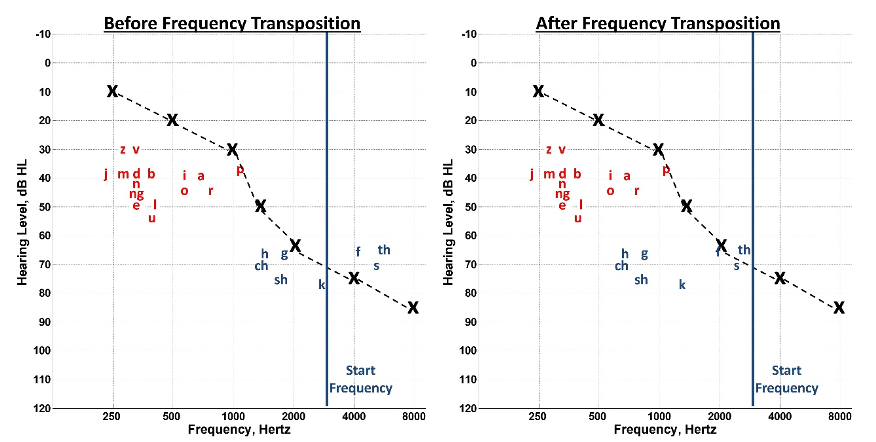
Figure 18. Illustration of frequency transposition in the same manner as Figure 16. This approach involves a ‘copy-and-paste’ technique where high-frequency components (in blue) are replicated and moved to a lower frequency range below the start frequency.

Figure 18 represents the same problem as depicted in Figures 3 and 16 but uses frequency transposition as a solution. In contrast to the start frequency for compression techniques, one manufacturer defines the start frequency for transposition as the point where all sounds are moved below. It can be thought of as the start of inaudibility or the regions on the cochlea that are no longer responsive to sound — that is, cochlear dead regions. Unlike frequency compression, the sounds are picked up and moved lower in frequency with transposition. There is not necessarily a compression of the source frequency; instead, only a band of energy with the highest intensity in the source region is usually moved down into a lower frequency. Also, transposition-like techniques can move sounds to a slightly lower frequency range because the high-frequency sounds are placed in the same regions as existing low-frequency sounds. As discussed later, frequency compression techniques are limited by low-frequency harmonics, usually below 1500 Hz or so. If the harmonics of voiced speech are moved below this, hearing aid users may complain about unpleasant sound quality. In contrast, with frequency transposition, the low-frequency sounds in the original signal are unaltered. However, one concern with transposition is masking the existing low-frequency sounds with the newly lowered high-frequency sounds.

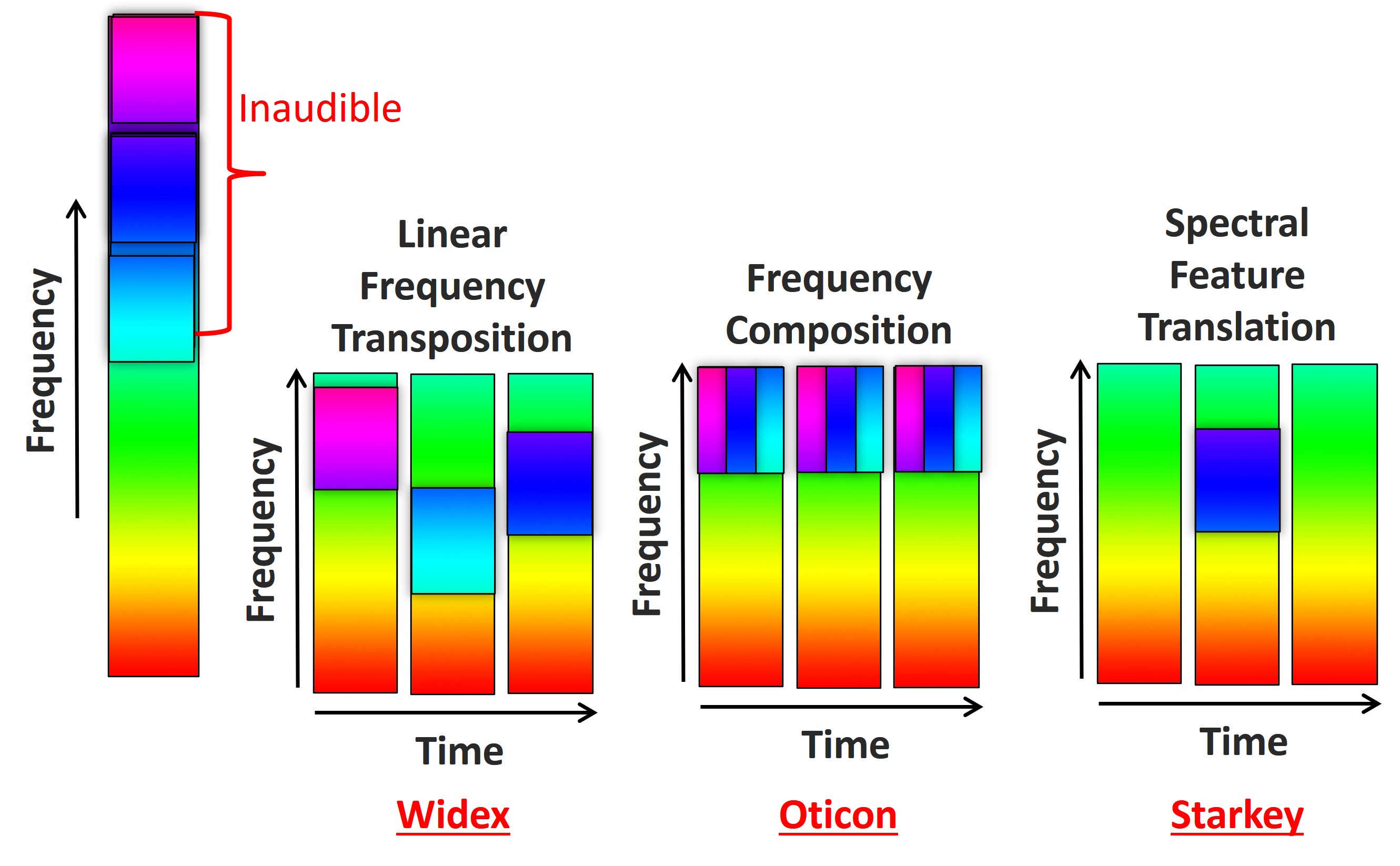
Figure 19. Schematic of the frequency transposition approaches in hearing aids in the same manner as in Figure 17. Widex employs linear frequency transposition, copying and pasting the highest intensity band from the source region (left color bar) to lower frequencies without compression, resulting in a linear shift in Hertz. Oticon’s method divides the source into bands (three in this example), merging them into a single output frequency space, thus overlapping rather than compressing them. Starkey’s approach, once known as spectral feature translation, selectively translates significant speech energy from high to low frequencies, activating only when detecting specific speech features, unlike the continuous transposition of the Widex and Oticon methods.

Figure 19 illustrates the differences between the frequency transposition methods used in hearing aids today. The transposition technique by Widex searches the input (color bar on the left) across time for the highest intensity band in the source region, copies a frequency range around that band, and then pastes it to lower frequencies without compressing it. This technique is called linear frequency transposition because sounds are shifted down by a linear factor in terms of Hertz. A band from the source is always lowered regardless of how soft it is. In addition, as shown, it picks up different parts of the source spectrum over time, depending on the input.

The transposition technique by Oticon, I call frequency composition. Oticon does not favor this terminology, but I like it because it nicely summarizes what the technique accomplishes. First, the technique divides the source region into two or three bands (three bands are shown in the figure). Then, unlike Widex’s linear frequency transposition, it combines all these bands and puts them in the same frequency space in the output. In this sense, it is multilayered frequency transposition. I call it composition because it is also like compression in that it takes a wide range of frequencies in the input and puts them in a smaller range in the output; however, instead of individually squeezing these frequency bands, it overlaps them.

The transposition technique by Starkey was once known as spectral feature translation. It is like the Widex technique because it finds when and where significant speech energy exists in the high frequencies. Then, when and where it detects it, it moves it to a lower frequency using the existing energy already in the low-frequency bands. But, unlike the other two techniques, it does not always lower something; instead, it will only lower frequency when it detects a spectral feature of speech.

Comparison of Techniques

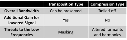
Table II. Summary of key differences between transposition and compression techniques in frequency lowering.

Table II summarizes the broad differences between the transposition and the compression techniques used for frequency lowering. Concerning the overall bandwidth, all transposition techniques allow the audiologist to select an option to keep the original, unlowered signal so that the bandwidth after frequency lowering is activated is the same as before it was activated. However, if you put the destination region close to the maximum audible output frequency, you can turn this option off since users cannot hear it. In contrast, compression techniques lower the original high-frequency sounds, meaning no high-frequency sound is above the lowered signal. Therefore, with these techniques, you must be careful not to have too much compression, which could reduce the audible bandwidth you had to begin with.

All the transposition techniques have a separate handle to adjust the gain of the lowered signal. I will call this the mixing ratio because transposition mixes the frequency-lowered signal with the original source signal. It is a delicate balancing act between making the lowered sounds perceptually salient so that the user can hear them versus having them so intense that they pop out of the perceptual stream and become segregated from the rest of the speech signal. This is an unnecessary option with the compression techniques because the signals are not mixed.

As noted earlier, with transposition, one threat to the low frequencies is that you risk moving some high-frequency masking noise into the region where there is existing low-frequency speech information. One of the concerns with compression is the risk of altering formant frequencies and their transitions. In addition, depending on how low you start the frequency compression, you risk altering the harmonics, resulting in unpleasant sound quality for the hearing aid user.

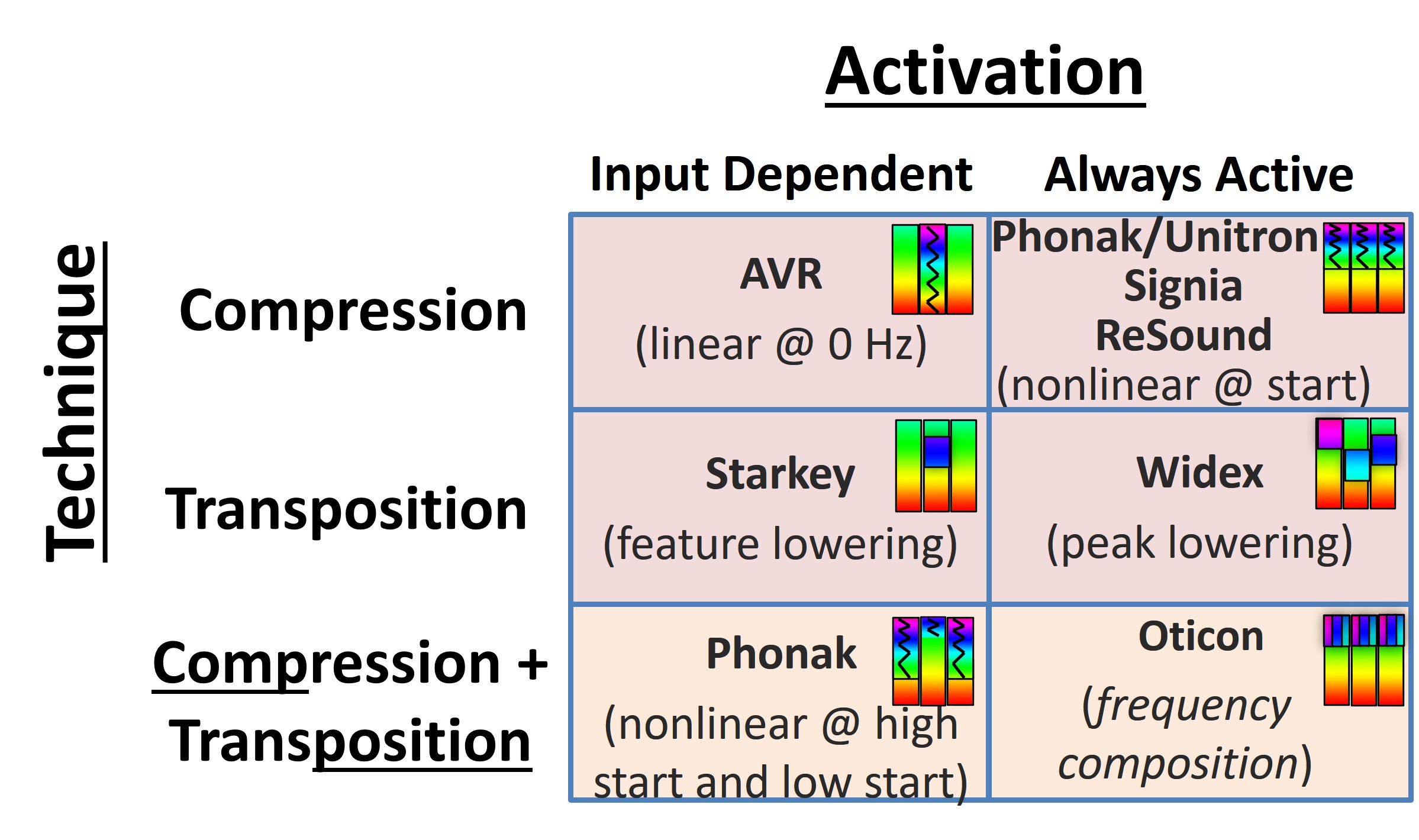
Figure 20. Summarizes all the frequency-lowering methods used by individual manufacturers (see text for details).

Figure 20 summarizes all the frequency-lowering methods used by individual manufacturers. One way of classifying the different strategies is whether or not frequency-lowering depends on the input (first column) or if they are always active (second column). The rows correspond to the specific techniques I just discussed: compression, transposition, and hybrid techniques between the two.

Starting with the upper-left is AVR Sonovation, which is no longer in business. However, I have included them for completeness. They made the first commercial digital hearing aid with frequency lowering. Whenever it detected significant high-frequency energy, it would go into full-on compression.

Then, there is the nonlinear frequency compression from Phonak, Unitron, Signia, and ReSound. As I already discussed, frequency lowering is always active with this strategy. It does not depend on the input, so the same frequency reassignment is maintained across time. The same goes for Widex; it is always active, continually lowering something — speech, noise, etc. Starkey, however, as indicated, lowers sound only when it detects there is a likelihood of a speech feature in the high-frequency source region.

Next, with Oticon, I have discussed why I put it in the category of compression and transposition. I use the term “composition,” which I borrowed from one of their subsidiaries. It, too, is always active and is continually lowering something. Furthermore, its behavior does not depend upon the input. It is like a hybrid compression type because it takes three source bands corresponding to different frequency ranges and puts them into a smaller range in the output. This contrasts with Widex and Starkey, who maintain the bandwidth of the lowered sounds in the output.

Finally, Phonak’s newest strategy in the lower left is adaptive nonlinear frequency compression. It depends on the input, so high-frequency dominated sounds can go lower in frequency with less compression, and low-frequency dominated sounds can have a higher cutoff to help preserve the formants and harmonics. I put this strategy in the compression and transposition category because it uses transposition to shift the compressed high-frequency dominated sounds even lower in frequency.

Widex Frequency Lowering

Part IV focuses on Widex’s linear frequency transposition, a feature in their hearing aid known as the Audibility Extender. In 2006, Widex was the first hearing aid company to offer frequency lowering in its main product line. This started a ten-year trend in which each major manufacturer would distribute one or more versions of frequency lowering.

Start Frequency

As with all frequency-lowering techniques, linear frequency transposition first divides the spectrum into a source region and a target or destination region. The source region is the frequency region where information is moved from. The target region is the frequency region where the lowered information is moved to. The start frequency can be considered the start of inaudibility or a dead region because the action happens below the start frequency, and everything above it is a candidate for frequency lowering. It is imperative to know the distinction between how the start frequency is used with this method compared to others. For example, with frequency compression techniques, all of the action happens above the nominal start frequency, which is also called the cutoff frequency or F min. Widex’s actual start frequency is about a half-octave below the nominal start frequency. Therefore, in this example, the nominal start frequency is 2500 Hz, and the actual start frequency is around 1800 Hz. Furthermore, the actual source region extends an octave above the nominal start frequency, which is 5000 Hz in this example.

Frequency Lowering Method

Over short time intervals, the algorithm continually searches for the most intense peak in the source region. Wherever it finds this peak, it creates a one-octave wide filter centered around it. Then, it lowers the entire filtered region one octave down into the target region. That is, the algorithm divides the frequencies in the filter by a factor of two and copies them down, so the original peak is maintained along with its lowered copy.

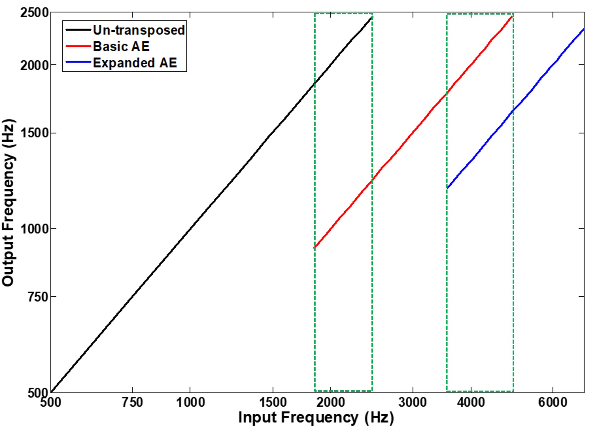
Figure 21. Input-output functions illustrating the action of Widex’s frequency lowering. The x-axis represents input frequencies, while the y-axis represents output frequencies. The black line corresponds to the un-transposed signal, showing no frequency change. The red line represents the basic Audibility Extender mode, with input frequencies halved in the output. Overlapping frequencies between transposed and un-transposed signals are denoted by green boxes. The blue line represents the expanded Audibility Extender mode, starting half an octave higher with output frequencies at one-third of the original input. Overlap between the un-transposed and transposed signals from the basic mode is maintained, resulting in peaks appearing two or three times in the output.

Figure 21 shows the action of Widex’s frequency lowering in terms of input-output functions. Frequencies going into the hearing aid are shown on the x-axis, and frequencies coming out are shown on the y-axis. The black line shows the un-transposed signal, for which you can see the frequencies coming into the hearing aid are the same in the output. The red line shows the transposed signal for the basic Audibility Extender mode. Notice that the nominal start frequency of the source region is 2500 Hz, but the actual start frequency is a half-octave lower, around 1770 Hz. The source region extends for an octave above the nominal start frequency, which is 5000 Hz in this case. Also, notice that the output frequencies associated with the red line are exactly half of the input frequencies, so 2000 Hz comes out at 1000 Hz, 3000 Hz comes out at 1500 Hz, 4000 Hz comes out at 2000 Hz, and so on. The green boxes show areas of overlap between the transposed and un-transposed signals. These frequencies will show up twice in the output: once at their original frequency and then again at their transposed frequency. 

The blue line shows the transposed signal in the expanded Audibility Extender mode. First, notice that its source region starts a half-octave above the nominal start frequency, around 3500 Hz. This is also a full octave above the start frequency for the source region of the basic Audibility Extender. The source region for the expanded Audibility Extender extends an octave above its start frequency, which is 7000 Hz. Furthermore, its output frequencies are 1/3 of the original input, so 4500 Hz comes out at 1500 Hz, 6000 Hz at 2000 Hz, and so on. It is also important to note that the un-transposed signal and the transposed signal from the basic audibility extender are both maintained when the Audibility Extender is in expanded mode, so just as before, as indicated by the green box, there will be overlap between the transposed signal in expanded mode, the transposed signal in basic mode, and some cases even the un-transposed signal. Therefore, peaks at these frequencies will show two or even three times in the output!

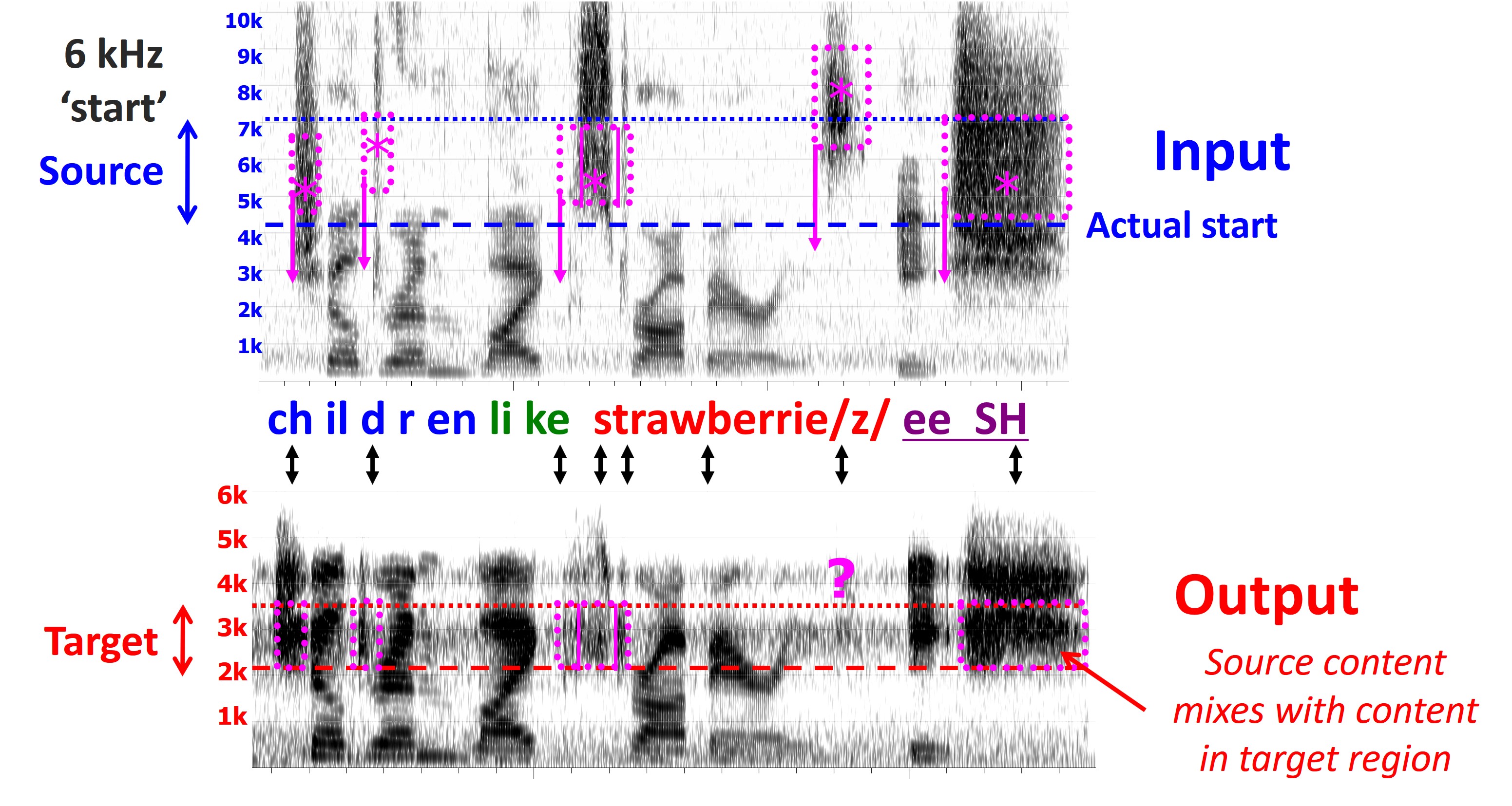
Figure 22. Spectrograms comparing the input and output of a hearing aid with frequency transposition, demonstrating the lowering of high-frequency sounds from the source region to the target region. Magenta boxes highlight indications of lowered information, while the question mark suggests energy beyond the device’s input range. The resulting output represents a mixture of source and target region energy.

The top spectrogram in Figure 22 shows the input to a hearing aid with frequency transposition, and the bottom shows the spectrogram of the output. The sentence is “children like strawberries,” followed by “eeSH,” one of the test stimuli I frequently use in my research. This sentence is useful because it has a lot of high-frequency energy associated with the fricatives, like “s” and “z,” the affricates, and the stop consonants. These sounds are indicated by the arrows. The nominal start frequency in programming software was set at 6 kHz. However, as you now know, the actual start frequency is really a half-octave lower at around 4200 Hz. For this particular device, input was limited to about 7 kHz. Next, the most intense sounds within the source region are moved down to the target region, as indicated by the bottom spectrogram’s red lines. Recall that the frequencies of the sounds in the source region are divided by two in the target region. Also, recall that the algorithm continually searches for the most intense peaks in the source region and filters them before lowering them. The magenta boxes and asterisks are areas in the source region where I can see some indication that the information has been lowered by looking at the output spectrogram. The magenta boxes in the output spectrogram correspond to the sounds in the upper spectrogram after lowering. The question mark indicates that it is hard to see any indication of the “z” being lowered at that time, probably because the energy was beyond the input range of the device. Another important thing to note is that this energy in the source region is mixed with whatever existing energy is present in the target region, so what you see in the output and what the hearing aid user hears is a mixture of the two.

Possible Pros of the Method

The algorithm’s behavior is dynamic because the exact frequency range that is lowered depends upon the input spectrum. The algorithm continually searches the short-term input spectrum for a peak, which is lowered by a factor of two or three. Therefore, the peak will appear at different frequencies in the target region across time. The algorithm is also active from one time to the next, even if there is no prominent peak in the input. It has been argued that this is beneficial because it can minimize discontinuities in the output signal and inadvertent artifacts. Finally, because peaks are linearly shifted by an integer factor (2 or 3), the harmonics within the peak will be generally maintained after lowering. The motivation behind this is to help promote a more natural and pleasant sound quality. As indicated earlier, only a portion of the spectrum around the peak is transposed, specifically a one-octave-wide region. As long as the algorithm picks the frequency region with the most essential information, this can be beneficial because we do not have to worry about compressing the signal. It also helps limit the amount of space in the target region occupied by the lowered signal, further reducing the concern that the newly transposed high-frequency energy may mask the existing low-frequency information.

Possible Concerns of the Method

One possible concern is that the high-frequency speech spectrum is often characterized by diffuse energy across a wide range, possibly discarding potential information. The term ‘potential information’ is used because we are unsure what information people extract from the frequency lowered signal. In addition, mixing the transposed and un-transposed signals in the low-frequency region may cause some issues with masking. Furthermore, this can make segregating the newly introduced high-frequency energy from the original energy difficult. Finally, if the lowered peak is associated with noise instead of speech, then the signal-to-noise ratio of the existing low-frequency signal will decrease.

Enhancements to the Method

Frequency transposition came out in 2006. In 2015, Widex came out with some enhancements to their original algorithm to improve the naturalness of the frequency-lowered signal. One of these enhancements was a voicing detector. Voiced speech is characterized by a harmonic relationship of its component constituent frequencies. Therefore, when the algorithm detects voiced speech, it applies less gain than voiceless speech. The rationale is that voiced speech is naturally more intense than voiceless speech, so it will perceptually pop out of the speech mixture if it has too much gain after lowering. That is, it will not blend in naturally, so the newly introduced high-frequency energy will segregate from the low-frequency speech and will not sound like speech. On the other hand, voiceless speech may need additional gain to make it perceptually salient. Another enhancement was the addition of a harmonic tracking system. The idea is to keep track of the harmonics of the voiced phonemes from the source region to align them better with the harmonics already in the target region. When the harmonics of the mixed-signal align, more pleasant sound quality and improved naturalness are expected. The last point is critical because it is not true with all transposition techniques.

An additional enhancement that is also a property of the other transposition techniques is the ability to amplify the full bandwidth of the original source signal as you would typically do without frequency lowering. Ideally, this should not be an issue if you put the frequency-lowered signal at the edge of the hearing loss, where you lose audibility for the amplified output. Because the hearing aid user cannot hear that information anyway, the thought is to remove it from the output so you do not increase the risk of feedback. However, because we cannot always guarantee that the clinicians will put the transposition setting where it needs to be, the concern is that the bandwidth will be artificially reduced compared to what the hearing aid user had to begin with. This may result in adverse outcomes because you may do more harm than good. Therefore, even if the clinician chooses the wrong frequency-lowering setting, the hearing aid user will be more likely to perform as well as without frequency lowering. It also gives clinicians more options regarding where to put the lowered signal without concern about rolling it off above the lowered output.

Programming Software Settings

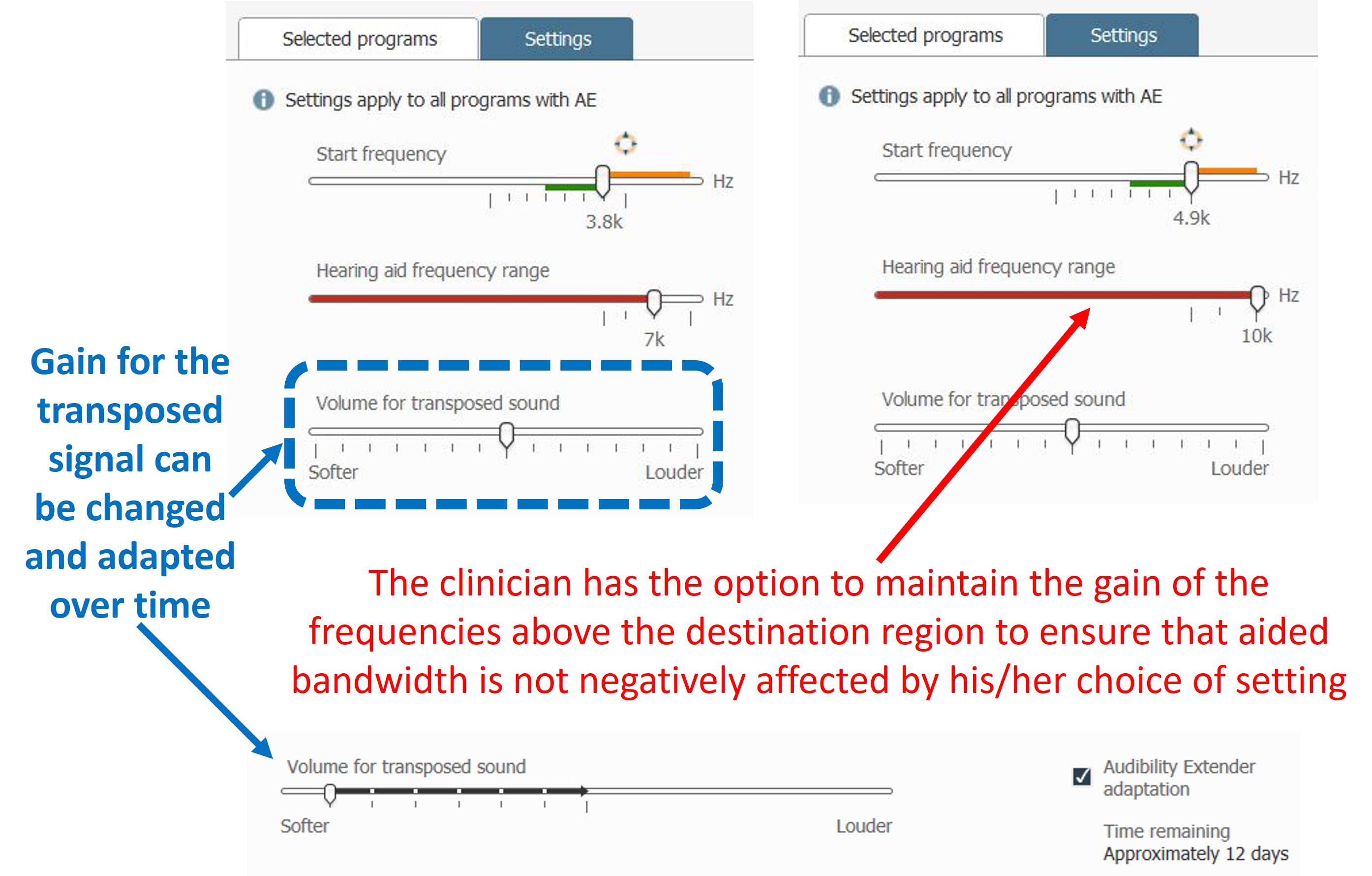
Figure 23. Screenshots from Widex COMPASS GPS version 4.5 illustrating settings for the Audibility Extender. The top shows a slider for selecting the start frequency, with options at 3.8 kHz and 4.9 kHz. The second slider, labeled “Hearing aid frequency range,” provides the ability to maintain the amplification of the original signal, ranging from the start frequency to the fullest bandwidth. The third slider, “Volume for transposed sound,” controls the relative gain of the lowered signal, aiming to balance audibility without distracting the user. The option to adapt the gain of the transposed signal over time is also available, allowing gradual adjustment to avoid overwhelming the user. The example indicates 12 days remaining to reach the final gain setting, adjustable via a slider.

Figure 23 shows screenshots from Widex COMPASS GPS version 4.5 of how the settings appear for the Audibility Extender. At the top is a slider corresponding to different start frequency selections. There are a finite number of settings. As you shift it to the right, you will increase the start frequency; as you shift it to the left, you will decrease the start frequency. With the fitting assistant, we are trying to optimize this setting based on the three goals discussed above. The screenshot on the left shows a start frequency of 3.8 kHz, and the one on the right shows a start frequency of 4.9 kHz.

The second slider is named “Hearing aid frequency range,” corresponding to the ability to maintain the original source spectrum. When Audibility Extender was first introduced, the hearing aid would roll off the frequency response above the start frequency. However, for reasons already discussed, clinicians can now maintain the amplification of the original signal. The option varies from the start frequency to its fullest bandwidth. As indicated before, if you know you are pretty sure what you are doing, you can keep this setting close to its lowest setting to minimize the likelihood of feedback.

The third slider is named “Volume for transposed sound,” corresponding to the relative gain of the lowered signal. All transposition methods offer this option because the lowered signal is mixed in with the existing low-frequency energy. One concern is that if it is too loud, it will perceptually segregate and pop out of the speech stream, distracting the hearing aid user. Likewise, if it is too low, the hearing aid user may not hear it.

Finally, you have the option to adapt the gain of the transposed signal over time. With adaptation, you can check the box and change the rate at which it will increase the gain for the lowered signal. You may want to gradually work the hearing aid user up the frequency lowering so the newly introduced information does not take them aback. This example shows approximately 12 days remaining for the hearing aid user to reach the final gain setting. You can change the adaptation rate by moving the slider.

Fitting Assistant: Goals

I created a fitting assistant to help clinicians make an informed decision when choosing a setting for the Widex Audibility Extender. The first step is to establish some goals. These goals may not be correct, but we must have some starting principles to work with. If there is some agreement in how the process is approached, then we can at least constrain some of the variability in how people are fit so that we can examine whether there are alternatives that will improve outcomes. The first goal is to choose the Audibility Extender setting that provides the most input bandwidth or information from the source region. The second goal is to minimize the overlap between the source spectrum of the unlowered and lowered signals so that the same input signal does not appear in the output at two different frequencies. This will be accomplished by choosing a higher start frequency. However, the start frequency should not be so high that gaps or holes exist in the input spectrum between the unlowered and lowered signals. These goals will be more apparent with the examples that follow.

Fitting Assistant: Example 1

This example is from Part II, which reviewed how to select the maximum audible output frequency, also known as the MAOF. In this example, the maximum audible output frequency was 4176 Hz. Remember that this indicates that sounds above this frequency will be inaudible for the hearing aid user with the chosen hearing aid when fit to prescriptive targets without frequency lowering activated. 

The fitting assistant is a tool to help inform and empower clinicians so you know what is happening underneath the hood so you can make more informed decisions. You can use this information to make the best selection based on those three goals established before.

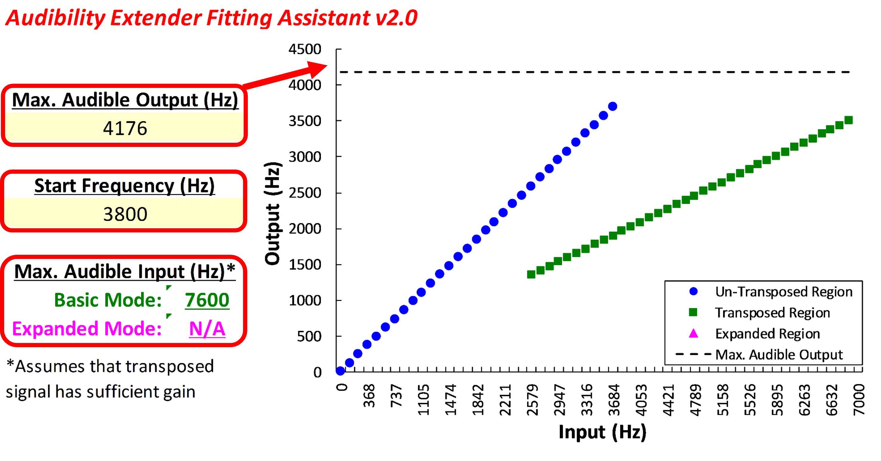
Figure 24. Screenshot of the Audibility Extender Fitting Assistant for Example 1. The yellow boxes allow input for the maximum audible output frequency (4176 Hz) and the start frequency (3800 Hz). The graph displays input frequencies on the x-axis and corresponding output frequencies on the y-axis. The blue line represents the un-transposed signal, while the green line indicates frequencies above 2700 Hz being transposed by a factor of 2 in the output. The horizontal dotted line visually depicts the maximum audible output frequency, serving as a bandwidth indicator. The maximum audible input frequency is reported as 7600 Hz, highlighting the expanded audible input bandwidth achieved through frequency lowering.

Figure 24 shows a screenshot of the Audibility Extender Fitting Assistant for Example 1. In the first yellow box, you enter the maximum audible output frequency, 4176 Hz. The dotted line on the graph corresponds to whatever you type into this maximum audible output box. This line serves as a visual indicator of how much bandwidth you have to work with. In the second yellow box, you enter the start frequency from the manufacturer’s software. The first start frequency I tested was 3800 Hz. The plot shows the frequencies going into the hearing aid on the x-axis and where they go in the output on the y-axis. The blue line is for the un-transposed signal. The green line shows how frequencies above 2700 Hz or so are transposed in the output by a factor of 2. The green line extends to 7600 Hz on the x-axis, which is reported as the maximum audible input frequency in the lower left. One goal is to maximize the audible input bandwidth. So with this setting, we have 7600 Hz, whereas the hearing aid user could only get information up to 4200 Hz without frequency lowering. However, this perhaps is not a good option because we are leaving a little bit off the table since we have about 400 Hz more to work with in the output (3800 Hz vs. 4176 Hz). It may not be that big of a deal, but if we can at least make full use of this range, we might as well do that. Selecting a lower start frequency will worsen this problem, so the only option is to try a higher start frequency.

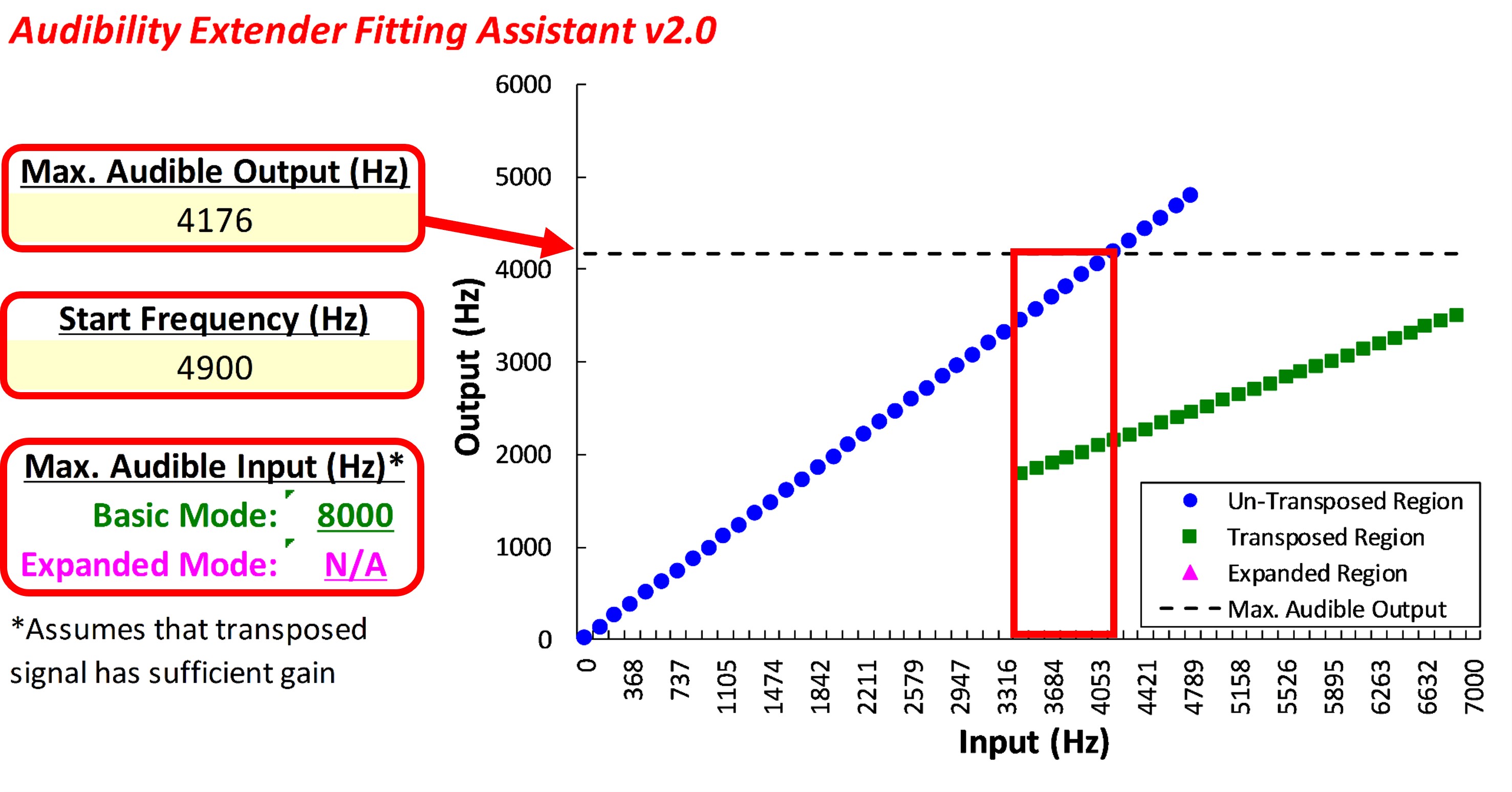
Figure 25. Screenshot of the Audibility Extender Fitting Assistant for Example 1 but with a 4900-Hz start frequency. The red box indicates the overlap between the un-transposed and transposed signals, which is less than the overlap seen with the 3800-Hz start frequency. Since a higher start frequency is unavailable, this is the optimal setting for the reported 4176-Hz maximum audible output frequency.

The other setting I explored is a 4900-Hz start frequency, as shown in Figure 25. We cannot test higher start frequencies because the option does not exist in the manufacturer’s programming software, as shown in Figure 23. Again, the un-transposed signal is shown by the blue line, and the transposed signal by the green line. This time, the maximum audible input frequency is 8000 Hz. We also want to look for gaps and overlap in the input between the blue and green lines. In this case, we have overlap between the two signals, as shown by the red box. This means that a single frequency coming into the hearing aid along this portion of the x-axis will come out at two frequencies, once at its original frequency — the blue line — and again at the transposed frequency — the green line. Compared to the 3800-Hz start frequency, with the 4900-Hz start frequency, there is less overlap and full use of the audible bandwidth; therefore, the 4900-Hz start frequency is the best option for this MAOF. Since a higher start frequency is not available, overlap is unavoidable. The following example will demonstrate a situation with a gap between the signals.

Fitting Assistant: Example 2

This second example from Part II corresponded to a maximum audible output frequency of 2700 Hz. The settings I will go through are ones that I picked out from what was available in the programming software. When you think you have found the best setting, you want to explore the range of settings by choosing one setting above and one below to ensure that you have optimized your goals.

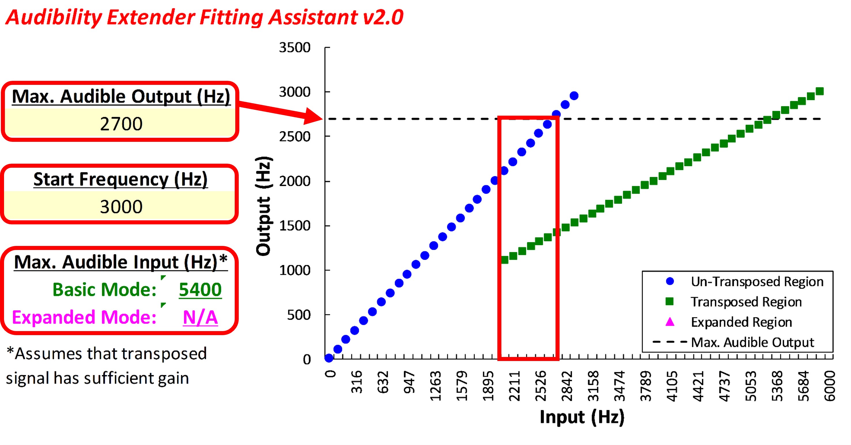
Figure 26. Screenshot of the Audibility Extender Fitting Assistant for Example 2 with a 2700-Hz MAOF and 3000-Hz start frequency. Notice that the horizontal line is now at 2700 Hz, again indicating how much audible bandwidth we have to work with. The red box indicates overlap between the un-transposed and transposed signals, which should be minimized.

The first setting I tried was a start frequency of 3000 Hz, as shown in Figure 26. For this setting, the maximum audible input is 5400 Hz, corresponding to where the green line crosses the dotted line; that is, where we lose audibility for the transposed signal. Notice the amount of overlap here shown by the red box. Recall that one goal is to minimize this overlap, if possible. Therefore, since we will have more overlap if we choose a lower start frequency, we will explore higher start frequencies. 

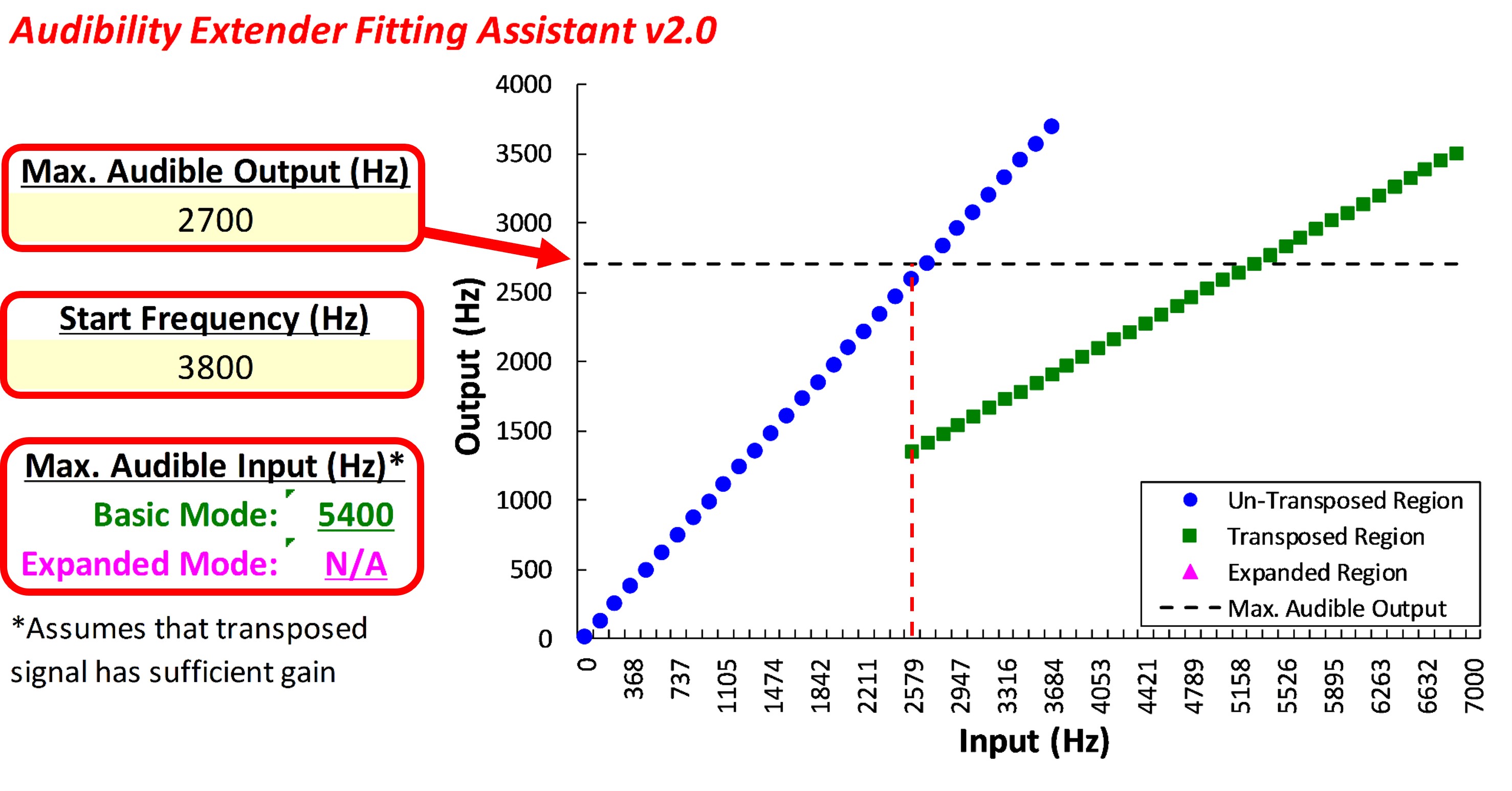
Figure 27. Screenshot of the Audibility Extender Fitting Assistant for Example 2 with a 3800-Hz start frequency. As indicated by the red vertical line, there are no gaps and almost no overlap between the un-transposed and transposed signals, making this an ideal setting for a 2700-Hz MAOF.

Figure 27 shows the next highest setting with a start frequency of 3800 Hz. Notice that the maximum audible input frequency is the same as before, 5400 Hz. Notice the input frequencies for the un-transposed and transposed signals BELOW the black dotted line corresponding to the MOAF. This is an ideal setting because at the frequency where we lose audibility for the un-transposed signal (where the blue line crosses the dotted line, as indicated by the red vertical line), it picks right up with the transposed signal, so there are no gaps, and there is almost no overlap.

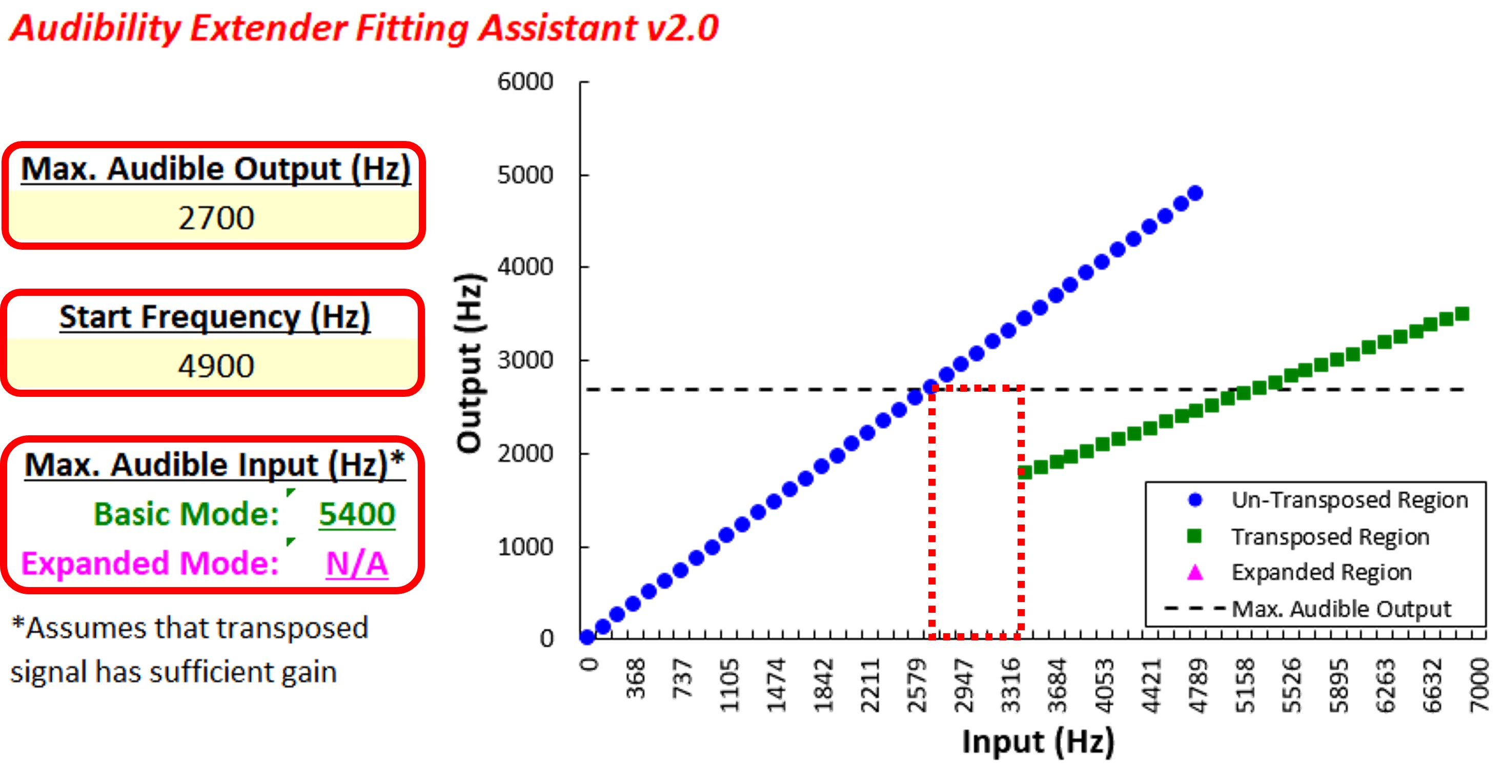
Figure 28. Example 2, with a 4900-Hz start frequency, illustrates a condition to avoid. The dotted red box reveals a gap in audibility: The un-transposed signal loses audibility at 2700 Hz, while the audibility for the transposed signal begins around 3400 Hz, resulting in a gap in the represented input frequencies in the output.

Figure 28 shows the output for the next highest start frequency, 4900 Hz, demonstrating one of the conditions we want to avoid. This time, the input frequency range shown by the dotted red box corresponds to a gap. This is because we lose audibility for the un-transposed signal at 2700 Hz, but we do not pick up audibility for the transposed signal until around 3400 Hz. So, there is a gap in the input frequencies represented in the output.

A Few Caveats about using the Fitting Assistant with Transposition

With frequency compression techniques, there is more or less a one-to-one ratio relationship between the output to the input. So, we know how much audibility we have for the input signal by simply looking at the audibility of the output and working backward using the fitting assistant. However, with transposition, the lowered is mixed with the un-lowered signals. Therefore, it is hard to tell from the amplified output what portion corresponds to the original signal and what portion corresponds to the lowered signal. This is where the special speech signals discussed in Part II may help. Therefore, while the fitting assistant can indicate whether the transposed speech has been moved to a region where aided audibility is possible, it cannot specifically verify that the transposed speech is audible.

Starkey Frequency Lowering

Part V reviews how Starkey implements frequency lowering in their hearing aids. The older feature name Starkey used for frequency lowering was “Frequency lowering,” but now simply, “frequency lowering.” 

Frequency Lowering Method

Starkey’s frequency-lowering method might be best described as spectral envelope warping. Spectral feature translation is another name Starkey has used to describe its frequency-lowering algorithm. This term is applicable because the algorithm lowers frequency only when the high-frequency spectrum contains spectral features characteristic of speech. The conceptual premise is similar to the source-filter theory of speech production, whereby the speech signal can be separated into a harmonic or noisy source and a superimposing filter created by the shape of the vocal tract. Translation refers to re-coding high-frequency filter peaks at lower frequencies using the source signal created by the harmonics of voiced speech.

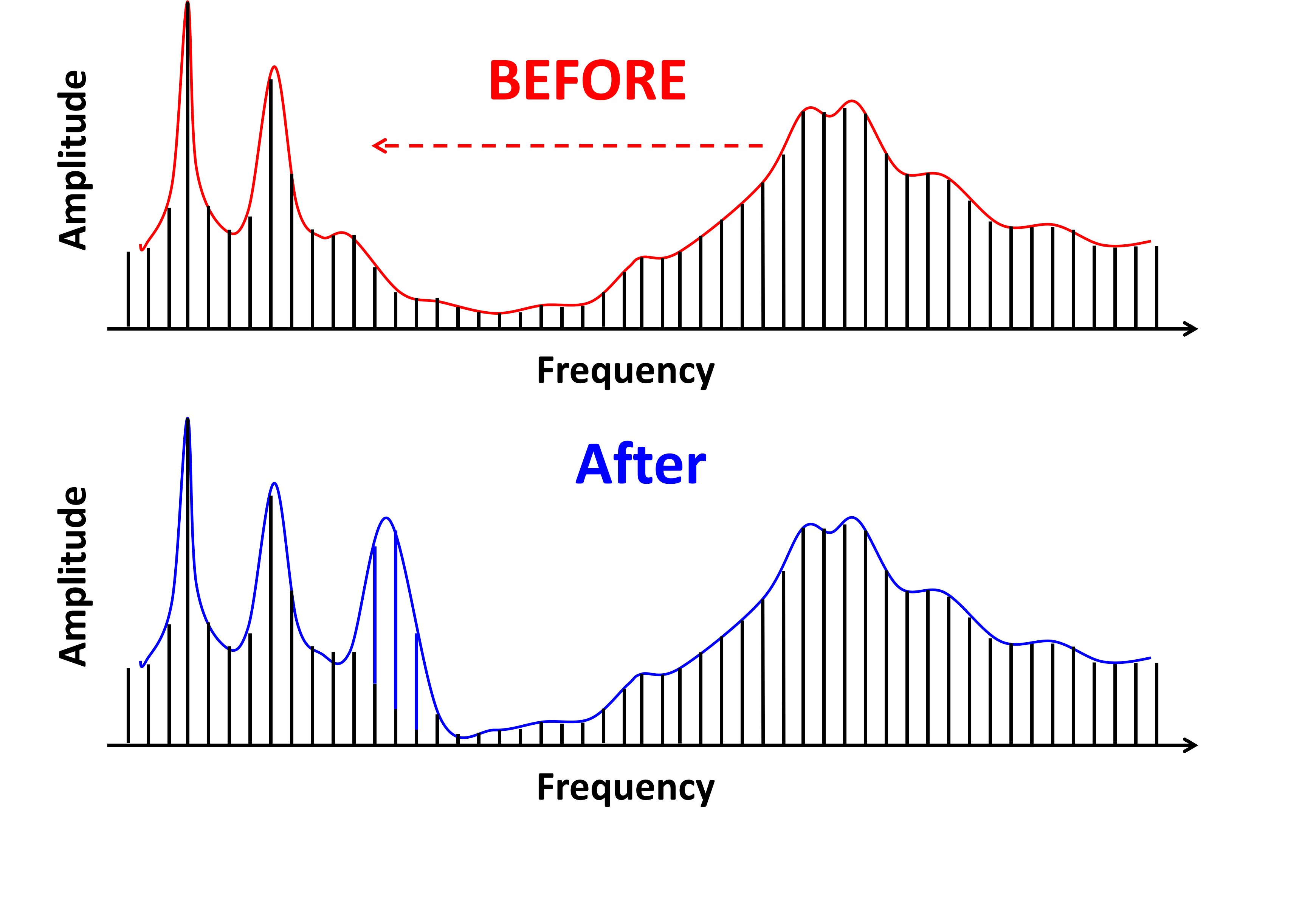
Figure 29. Illustration of the Starkey algorithm for frequency lowering. The top of the figure shows the separation of the speech signal into a source (voiced speech harmonics, black lines) and a filter (red line). The algorithm identifies high-frequency speech features (peaks) and translates them to lower frequencies. This is depicted at the bottom of the figure by the alteration of the filter (smooth blue line) and the increase in amplitude of the source harmonics (vertical blue lines) at lower frequencies. The original spectrum is preserved up to about 5700 Hz, ensuring the audible bandwidth is not reduced through the application of this technique.

As shown at the top of Figure 29, the premise of the Starkey algorithm is to separate the speech signal into a source signal and filter. The black lines correspond to the harmonics of voiced speech, which is the source, and the red line corresponds to the filter. The idea is to use the filter to find a high-frequency speech feature, namely a peak, and then translate it to a lower frequency. First, the algorithm starts with its original harmonic source (vertical black lines). Then, it alters the superimposing filter to recreate the high-frequency peak at a lower frequency (smooth blue line at the bottom of the figure). Finally, the source harmonics increase amplitude to create the new low-frequency peak (vertical blue lines at the bottom of the figure). Notice that up to a certain point, around 5700 Hz, the original spectrum is retained after lowering. This prevents the clinician from unintentionally harming the hearing aid user by restricting their audible bandwidth when misusing this technique.

Programming Software Settings

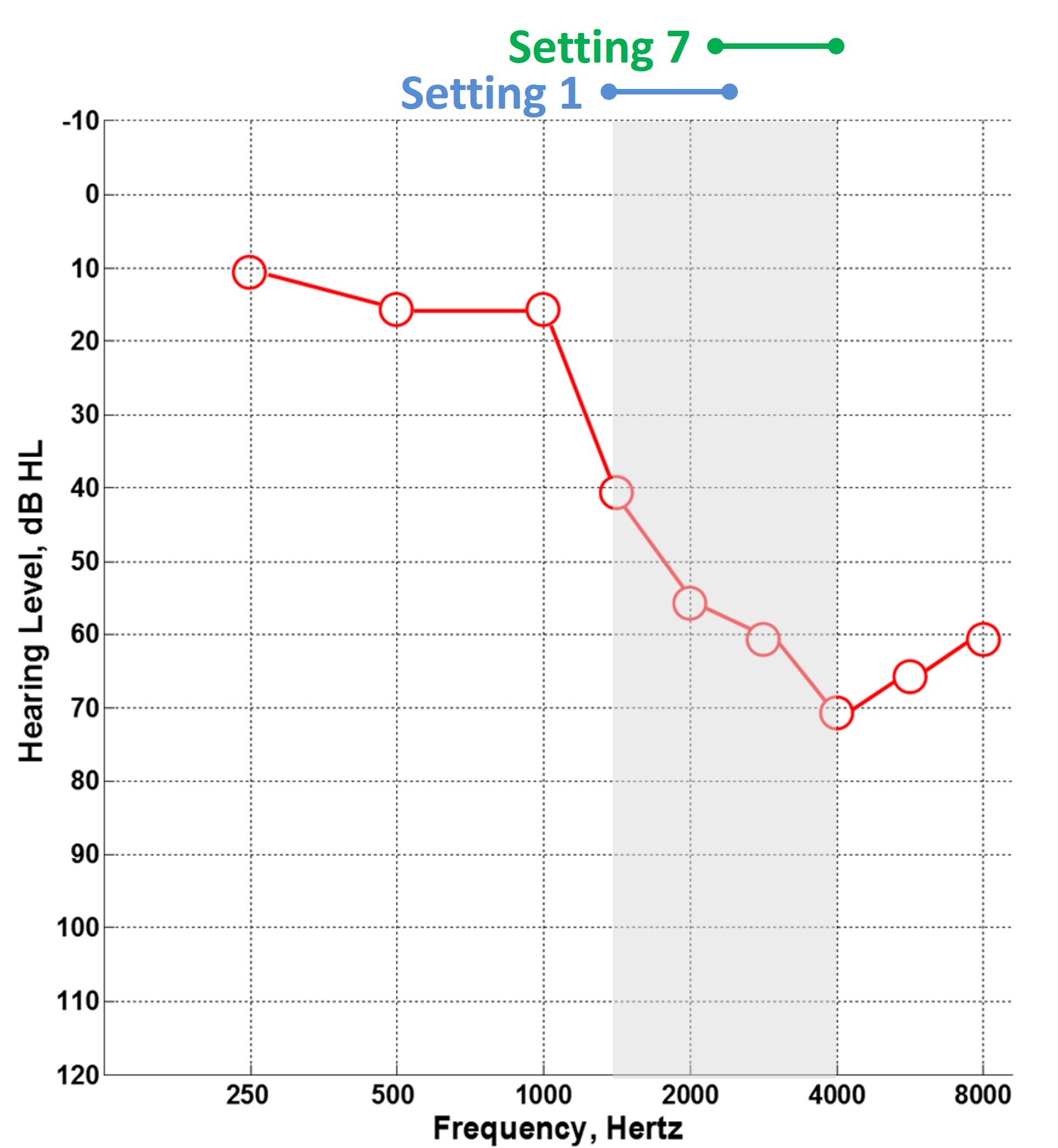
Figure 30. Audiogram illustrating the seven settings of the Starkey frequency-lowering algorithm (“frequency Lowering Bandwidth”), with the destination region indicated by the gray-shaded area between 1500 and 4000 Hz. Bandwidth setting 1 puts the destination at the lower end, while Bandwidth setting 7 puts it at the higher end of this range.

The Starkey frequency-lowering algorithm has seven different settings called “Frequency Lowering Bandwidth.” These settings put the destination region somewhere between 1500 and 4000 Hz, as shown by the gray-shaded region on the audiogram in Figure 30. For example, Bandwidth setting 1 puts the destination in the lowest part of the gray-shaded region, and Bandwidth setting 7 puts it in the highest part. As indicated by the audiogram, the general idea is to use frequency lowering to accommodate the slope of the audiogram. In particular, Starkey recommends that their algorithm be used only when the audiometric slope is at least 25 dB per octave. Ideally, the destination region frequency would begin at the frequency that starts the slope and end at the frequency where thresholds are greater than 70 dB HL. In the absence of probe microphone measures to determine the maximum audible output frequency, the rationale for these criteria is like the other transposition techniques: to put the lowered information near the edge of the audible spectrum.

Starkey has released several recommendations to maximize the likelihood that hearing aid users benefit from frequency lowering. As indicated, the first recommendation is that the audiogram has a slope of at least 25 dB per octave. The second is that the thresholds between 250 and 1000 Hz be less than or equal to 55 dB HL. The third is that at least one threshold between 1000 and 3000 should be at least 55 dB HL. The fourth recommendation concerns the default settings. If any threshold between 4000 and 8000 Hz is at least 55 dB HL, then the Bandwidth setting is number 3. If all the thresholds between these frequencies are at least 70 dB HL, then the Bandwidth setting is number 5.

Starkey frequency lowering will default to “ON” if both ears meet the candidacy criteria from the previous slide. If only one ear meets the criteria and the other is within 10 dB, they will default to “ON.” If one ear meets the criteria and the other is more than 10 dB better, it will default to “OFF.” And if neither ear meets the criteria, both will default to “OFF.” A unilateral fitting will default to “ON” for that ear if that meets the criteria and to “OFF” if it does not. Finally, if you indicate that you have a pediatric fitting, it will default to “OFF.”

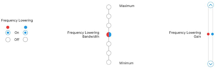
Figure 31. Starkey’s two controls for frequency lowering as displayed in the Pro Fit 2023.1 programming software. The first control, shown in the middle, sets the bandwidth of the source region, with seven Frequency Lowering Bandwidth settings ranging between ‘Minimum’ and ‘Maximum’ labels. On the right side of the figure, controls are provided for adjusting the gain of the lowered signal independently for the left and right ears, allowing for customized adjustments based on individual perceptual needs or preferences.

As shown in Figure 31, Starkey has two controls for frequency lowering. The first control determines the bandwidth of the source region. Also, as indicated, there are seven Frequency Lowering Bandwidth settings, but they are not labeled as such; instead, they are bounded will the labels “Minimum” and “Maximum.” Again, the default setting is determined by the audiogram entered into the programming software. It also determines the location of the destination region, which, as already indicated, encompasses the range somewhere between 1500 and 4000 Hz. Unfortunately, I have yet to figure out the exact mapping between the source and destination regions for each of the seven bandwidth settings, which is why I do not have a Fitting Assistant for this particular technique. The controls on the right are where you can adjust the gain of the lowered signal for the left and right ears. As mentioned in Part IV, the reason is that the lowered signal is mixed with the un-lowered signal; therefore, we must strike a balance. If the gain is too low, the lowered signal will not be perceptual salient, and if it is too high, it may perceptually segregate from the rest of the speech stream and become a distraction.

Demonstration of Algorithm Behavior

To help better understand the behavior of the Starkey algorithm, I created a series of speech-like sounds that systematically varied in frequency, which were then recorded through a Starkey hearing aid. The rationale was that if the algorithm is sensitive to speech, speech should be used as a stimulus. The series of stimuli consisted of a pair of vowels with a narrowband noise to simulate frication. The center frequency of the narrowband noise started low, so the stimulus sounded something like (“aa sh aa”). With each iteration, the center frequency of the noise band increased. Then, midway, the vowels changed to /i/ (“ee”), and the stimuli sounded like /isi/ (“ee see”).

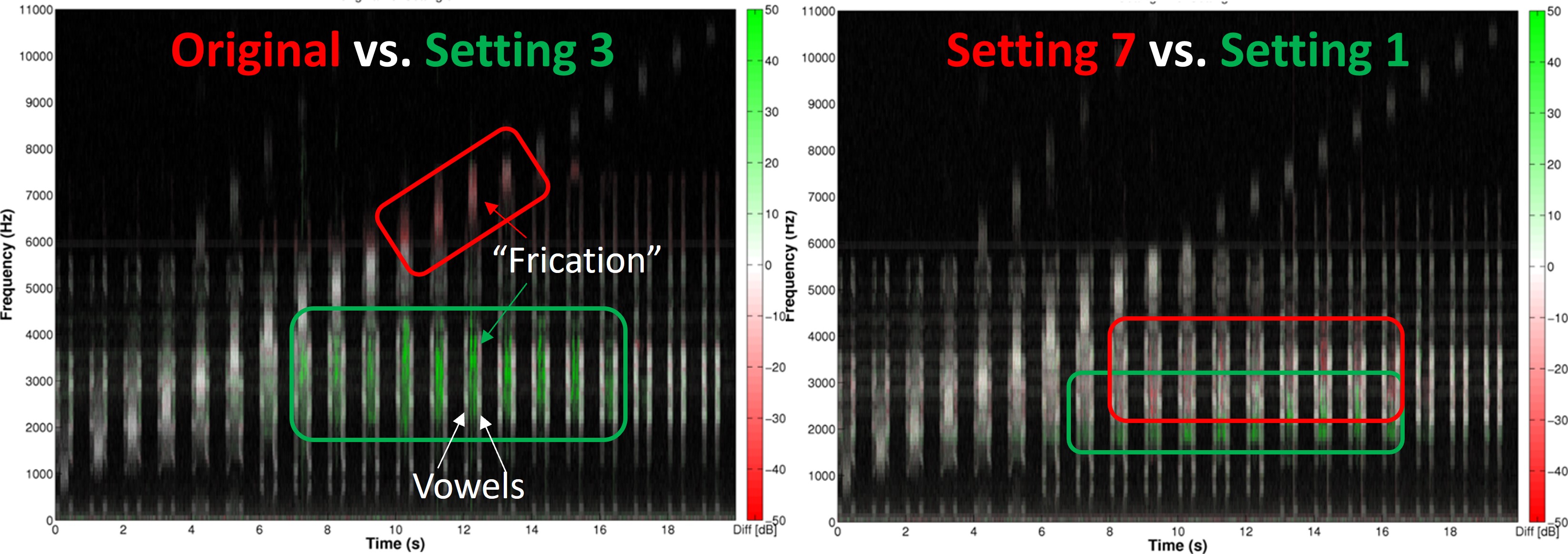
Figure 32. The left spectrogram contrasts original speech stimuli with those subjected to frequency lowering at a bandwidth setting of 3. Green shading indicates areas with more energy in the frequency-lowered stimulus, predominantly in fricative sounds. In contrast, white shading shows similar energy levels in lowered and un-lowered stimuli, particularly in vowels. The right spectrogram compares the effects of the maximum (setting 7) and minimum (setting 1) bandwidth settings. Here, green shading indicates areas where setting 1 has more energy, while red shading shows where setting 7 has more energy. This comparison illustrates that the main difference between bandwidth settings lies in the positioning of lowered information within the destination region, with lower frequencies affected in setting 1 and higher frequencies in setting 7.

The spectrograms in Figure 32 show each speech-like stimulus as a function of time wherever there is a burst of energy. The spectrogram on the left compares the original, un-lowered stimuli to frequency lowering with a bandwidth setting of 3. The parts shaded in green are where there is more energy for the frequency-lowered stimulus. The parts shaded in white are where the two are the same. Notice that energy in the vowels is the same for the lowered and un-lowered stimuli and that only the frication is lowered. Also, notice that lowering occurs only when the source signal has energy above 4000 Hz, which is about at the 7-second mark on the spectrogram. Also, notice that it stops lowering when the original source signal has energy above 9000 Hz, which is about the 17-second mark on the spectrogram. The parts shown in red are where the original signal has more energy than the frequency-lowered signal. Recall that Starkey’s frequency lowering will maintain the original speech signal up to 5700 and filter the energy above this.

The spectrogram on the right compares the maximum bandwidth setting, number 7, to the minimum bandwidth setting, number 1. Again, the parts where the two have the same energy are shown in white. This time, the parts in green are where bandwidth setting 1 has more energy than bandwidth setting 7 and the parts in red are where bandwidth setting 7 has more energy than bandwidth setting 1. The point here is that the primary difference between the frequency-lowering bandwidth settings is where the lowered information goes in the destination region, being lower for bandwidth setting 1 and higher for bandwidth setting 7.

Summary

In summary, Starkey’s algorithm is similar to Widex’s because only a portion of the high-frequency signal centered around a peak in the source region is lowered. However, its technique differs because it manipulates the harmonics in the low-frequency source spectrum. It is also dynamic because it engages frequency lowering only when it detects a peak in the source region. Like the other frequency transposition techniques, it mixes the lowered and the un-lowered signals. However, concerns about masking the existing low-frequency energy are lessened. This is because the algorithm engages only when it detects speech-like energy in the high-frequency spectrum. Furthermore, strong high-frequency speech cues tend to be exclusive of useful low-frequency information. Finally, as indicated earlier, Starkey’s algorithm is like all the transposition techniques because it retains the original high-frequency spectrum. However, it differs from the others because the clinician cannot control this property; instead, it keeps the original spectrum up to 5700 Hz for all frequency-lowering settings.

Oticon Frequency Lowering

Part VI provides a review of Oticon’s method of frequency lowering. It is a multilayered frequency transposition method that they call “Speech Rescue.”

Frequency Lowering Method

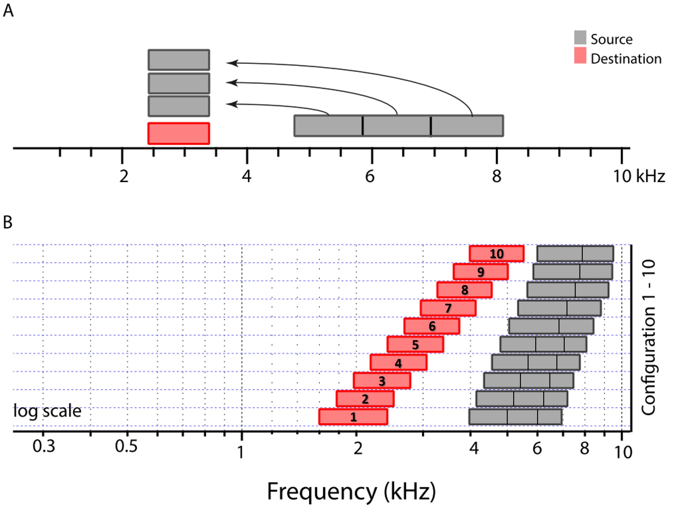
Figure 33. Oticon’s approach to frequency transposition divides the high-frequency source band into two or three sub-bands (represented by gray bars). These sub-bands are then recombined into the same location in the destination region (indicated by the red bar). This method differs from Widex and Starkey as the specific frequencies lowered remain constant over time. Stacking multiple source bands at identical output frequencies may cover a broader input frequency range while minimizing disruption to existing low-frequency elements like formants in the destination region. Oticon’s ten frequency-lowering configurations vary in source and destination frequencies; configurations 1-5 use three sub-bands, while configurations 6-10 use two, adapting the frequency transposition to different hearing needs.

As indicated in Figure 33, Oticon uses transposition to lower high-frequency information. However, they differ from other transposition techniques in that they divide the source band into two or three different sub-bands, as shown by the gray bars. Then, the sub-bands are recombined at the same place in the destination region, as shown by the red bar. Oticon’s frequency-lowering technique transposes information in the source region without compression. Recall this is how all the transposition methods work; they take some or all of the high-frequency spectral content in the source band and copy it down without squeezing it. However, the Oticon technique is like compression in that a wider range of input frequencies are mapped onto a smaller range in the output. This is why I call it composition.

Unlike the Widex and Starkey transposition techniques, the exact frequencies being lowered do not change over time. We can hypothesize about the advantage of stacking the individual source bands at the same frequencies in the output compared to other transposition techniques. One potential advantage is that the same output bandwidth can cover a wider range of frequencies from the input. In addition, minimizing its footprint in the destination region can minimize the disruption of existing low-frequency information already in the signal, like the formants.

Programming Software Settings

As indicated in Figure 33, Oticon offers ten different frequency-lowering settings, what they call configurations. The lowest configuration, 1, corresponds to the lowest source and destination frequencies. As shown by the gray bars, the source region is divided into three sub-bands for configurations 1 through 5 and two sub-bands for configurations 6 through 10. Notice the gaps between the red and gray bars, representing the gap between the destination and source bands. This is unlike Widex’s frequency transposition technique, where the source region abuts up to and overlaps with the destination region. Assuming that you put the destination region at the edge of the audible spectrum, these gaps correspond to a range of input frequencies for which there is no representation in the output, where we lose audibility. This might work because all of the source regions cover frequencies likely to carry some of the critical high-frequency information associated with frication.

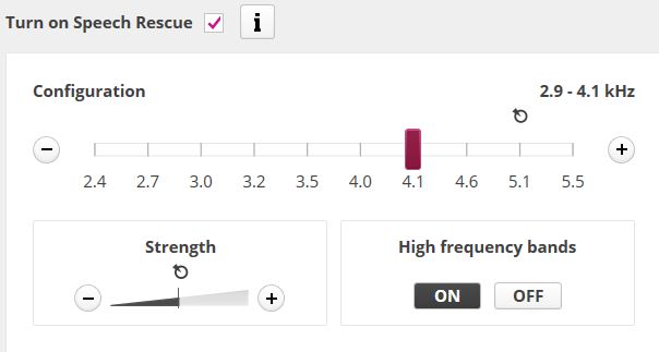
Figure 34. Display of the Speech Rescue settings in the Genie 2 | 2023.2 software by Oticon. Instead of numeric labels, the configurations are represented by the highest frequency of the destination region in kHz. The selection is made by adjusting a slider, with this specific example showing the settings for configuration 7. As indicated in the lower left, the software allows clinicians to adjust the gain (“strength”) of the lowered signal. The option in the lower right is to activate or deactivate the high-frequency bands above the destination region.

Figure 34 shows how the Speech Rescue settings appear in the manufacturer’s software (Genie 2 | 2023.2). Notice that the configurations are not numbered 1 through 10 but show the highest frequency in kHz of the destination region. Different configurations are selected by simply moving the slider. This example shows the setting corresponding to configuration 7.

Just as with all the transposition techniques, the clinician can adjust the gain of the lowered signal. Remember, this is important because it mixes the lowered signal with the original signal, so there is a need to balance perceptual saliency and perceptual segregation. That is, if the gain is too low, the hearing aid user may not notice the lowered signal, and if it is too high, it may pop out from the speech signal and become distracting.

Finally, the last option is to turn the high-frequency bands On or Off. Like all the transposition techniques, the clinician has the option to maintain the gain of the destination region above where there is frequency lowering. Furthermore, just as with the other transposition techniques, if you put the destination region right at the edge of the aided audibility, you might as well turn this gain off because you just run the risk of potentially introducing a feedback signal when you might not otherwise. However, you can think of this option as a fail-safe against choosing a frequency-lowering setting that is too aggressive, which would otherwise remove everything above the destination region, thereby reducing the audible bandwidth. If you choose the recommended configuration as discussed below, the hearing aid user should not hear the high-frequency bands above the destination region, so you might as well turn them off.

Demonstration of Algorithm Behavior

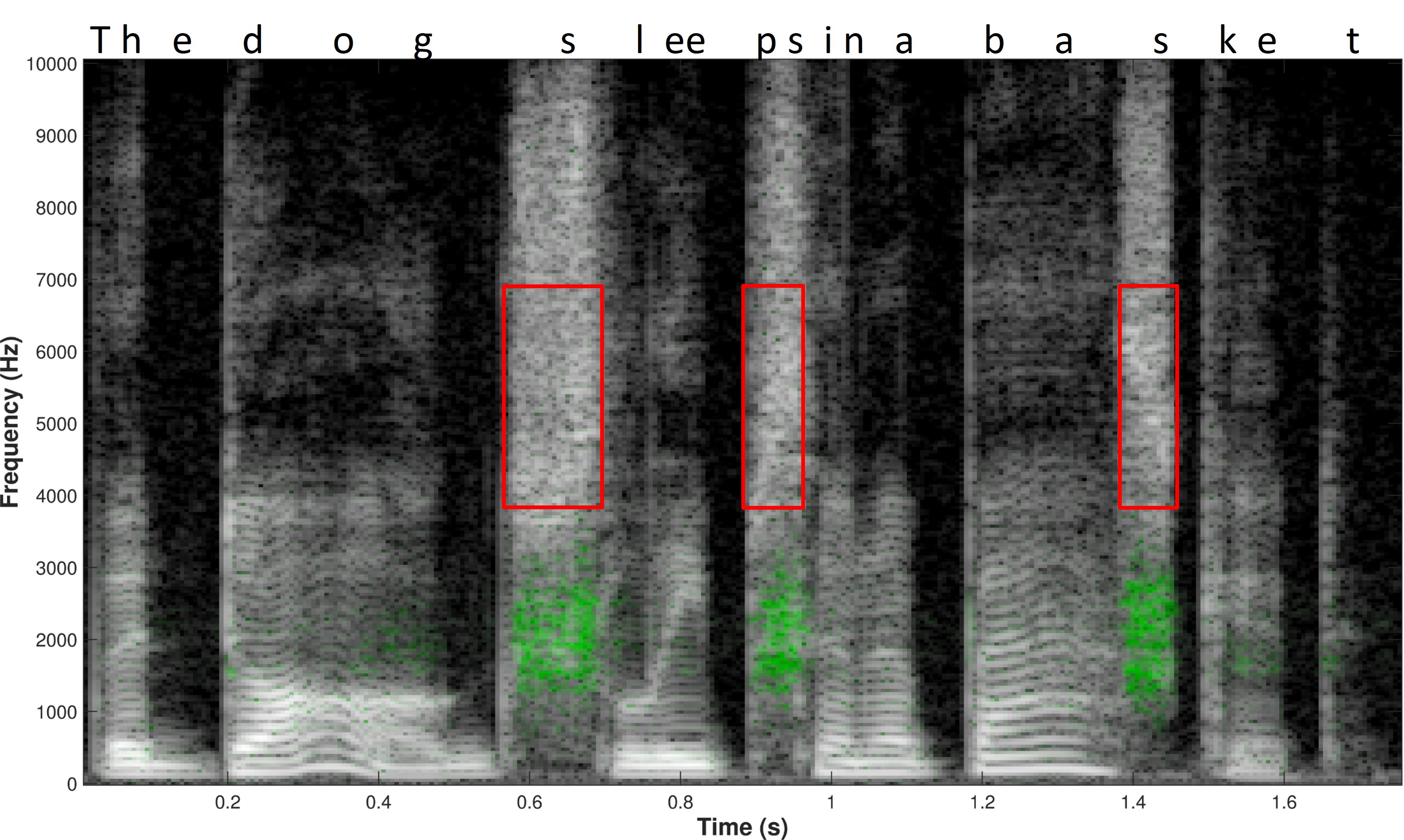
Figure 35. Spectrogram of the sentence “the dog sleeps in a basket” demonstrating the Speech Rescue feature in action. The x-axis represents time, and the y-axis indicates frequency, with the intensity of white pixels denoting energy levels at each frequency and time point. The red boxes highlight the source regions with the resultant lowered frequencies represented by green pixels.

To help see Speech Rescue in action, Figure 35 shows a spectrogram of the sentence “the dog sleeps in a basket.” Time is along the x-axis, and frequency is along the y-axis. The brightness of the white pixels indicates the amount of energy at each time and frequency. Notice that the energy in the high frequencies is mainly associated with the stop and fricative consonants and is spectrally broad. The red boxes correspond to the source of the frequency-lowered information shown by the green pixels. Be aware that while the algorithm is always on and lowering something that, like the Widex technique, sometimes there is just not enough energy in the source region for it to be seen when mixed with the original low-frequency signal.

Fitting Assistant: Goals

As with the other Fitting Assistants, we need to establish common goals grounded in First Principles. Again, we can argue whether these goals are right or wrong. But the purpose here is to establish some agreement regarding how we initially program our settings. Then, we can eventually evaluate whether or not this goal is the appropriate choice. The goal chosen for Speech Rescue is to put the destination region at the edge of the audible spectrum.

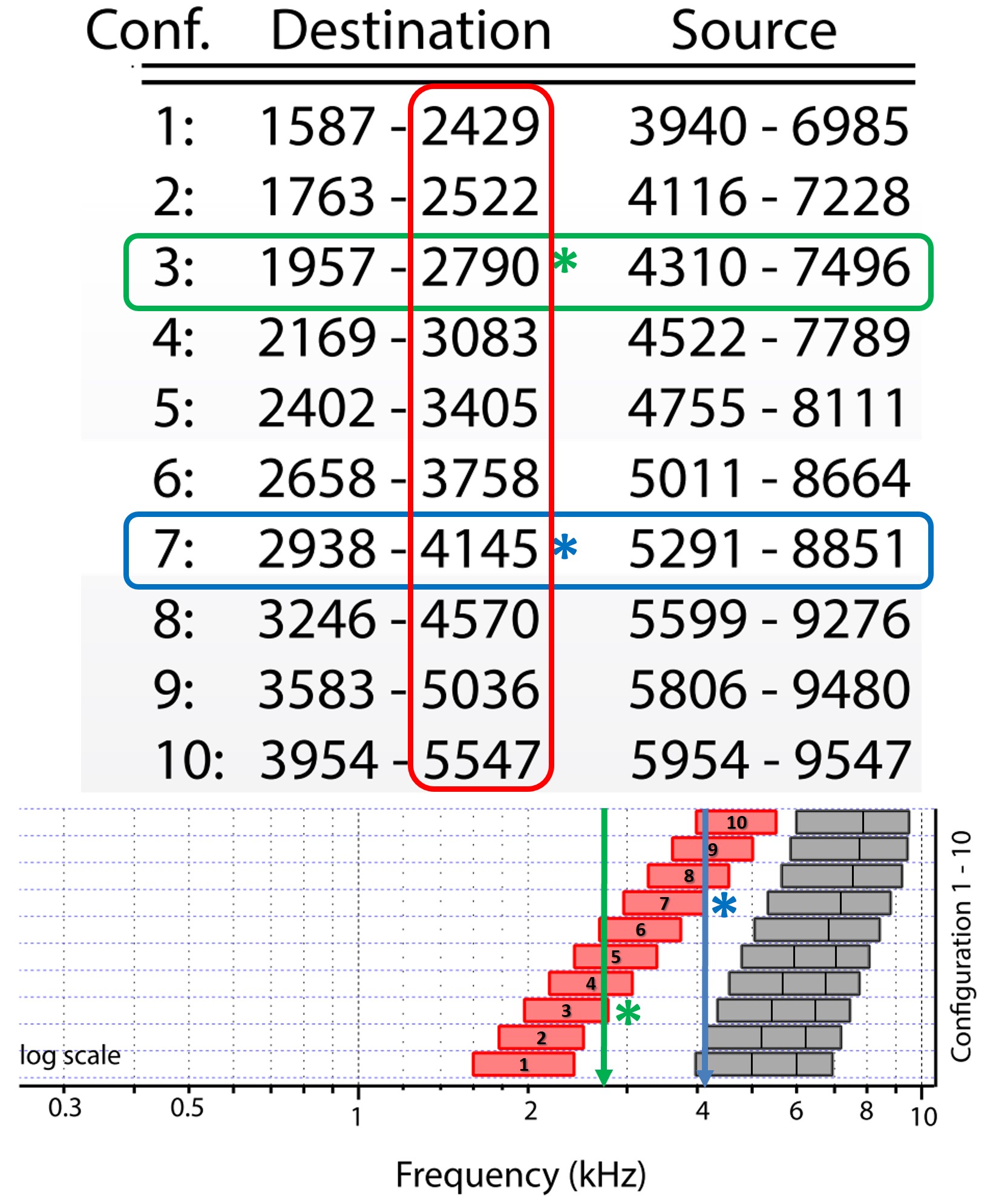
Figure 36. Table displaying destination and source region values for Oticon’s ten frequency-lowering configurations. The red box highlights the edge frequencies of the destination regions, which are essential for matching the Maximum Audible Output Frequency (MAOF). The fitting assistant recommends the optimal configuration based on inputting the MAOF, selecting the lowest configuration where at least 95% of the destination region falls below the MAOF. For an MAOF of 4176 Hz, as used in the initial audiogram example, configuration 7 is ideal, with a destination region ending at 4145 Hz. This is visually represented in the lower right plot, where the edge of the red bar aligns closely with the blue line (MAOF). In contrast, for an audiogram with an MAOF at 2700 Hz, configuration 3 is indicated as ideal, as shown by the alignment with the green line in the plot. This table and accompanying plot guide clinicians in choosing the most appropriate configuration for individual hearing aid users.

Figure 36 shows a table of values for the destination and source regions corresponding to the ten different configurations. The values in the red box correspond to the edge of the destination region. Essentially, we want to choose the configuration whose edge frequency for the destination closely matches the Maximum Audible Output Frequency. In fact, when you enter the MAOF into the fitting assistant, it tells you which configuration best matches this criterion. It chooses the lowest configuration for which at least 95% of the destination region is below the maximum audible output. Recall that the MAOF of the first audiogram we used throughout this article is 4176 Hz. According to our goal, configuration 7 is best, with a destination region ending at 4145 Hz. Our rationale can be visualized with the blue line representing the MAOF in the plot in the lower right. The best configuration will be the one where the edge of the red bar is close to the blue line, which is configuration 7. Similarly, with the example where we lost audibility at 2700 Hz, the ideal configuration according to this goal would be configuration 3. This is shown in the plot by the green line.

Fitting Assistant: Example 1

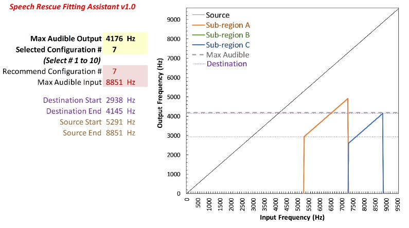
Figure 37. Display of the Fitting Assistant for Oticon’s Speech Rescue. The top yellow box allows the clinician to input the Maximum Audible Output Frequency (MAOF), based on which the assistant recommends an optimal configuration (shown in the red box) and indicates the highest input frequency that will be made audible. Upon entering a configuration number (configuration 7 in this example), the software plots frequency input-output functions with the source region divided into two sub-bands (orange and blue lines), both undergoing linear transposition to the same destination region. The gray horizontal line represents the MAOF, showing that most lowered information in this configuration will be audible.

Figure 37 shows the first example as it appears on the Fitting Assistant. When you enter the maximum audible output frequency in the yellow box at the top, it will provide you with the recommended configuration in the red box below, along with the highest input frequency that will be audible. Whatever configuration number you enter into the yellow box at the top will be plotted by frequency input-output functions, and the values corresponding to the destination and source regions will be reported to the left. For configuration 7 in this example, you can see that the source region is divided into two sub-bands, as shown by the orange and blue lines. Notice how each band undergoes linear transposition and that each sub-band occupies the same frequency region in the output. As with the other Fitting Assistants, the maximum audible output frequency is plotted with the gray horizontal line. So, as you can see, most of the lowered information will be audible with this configuration.

Fitting Assistant: Example 2

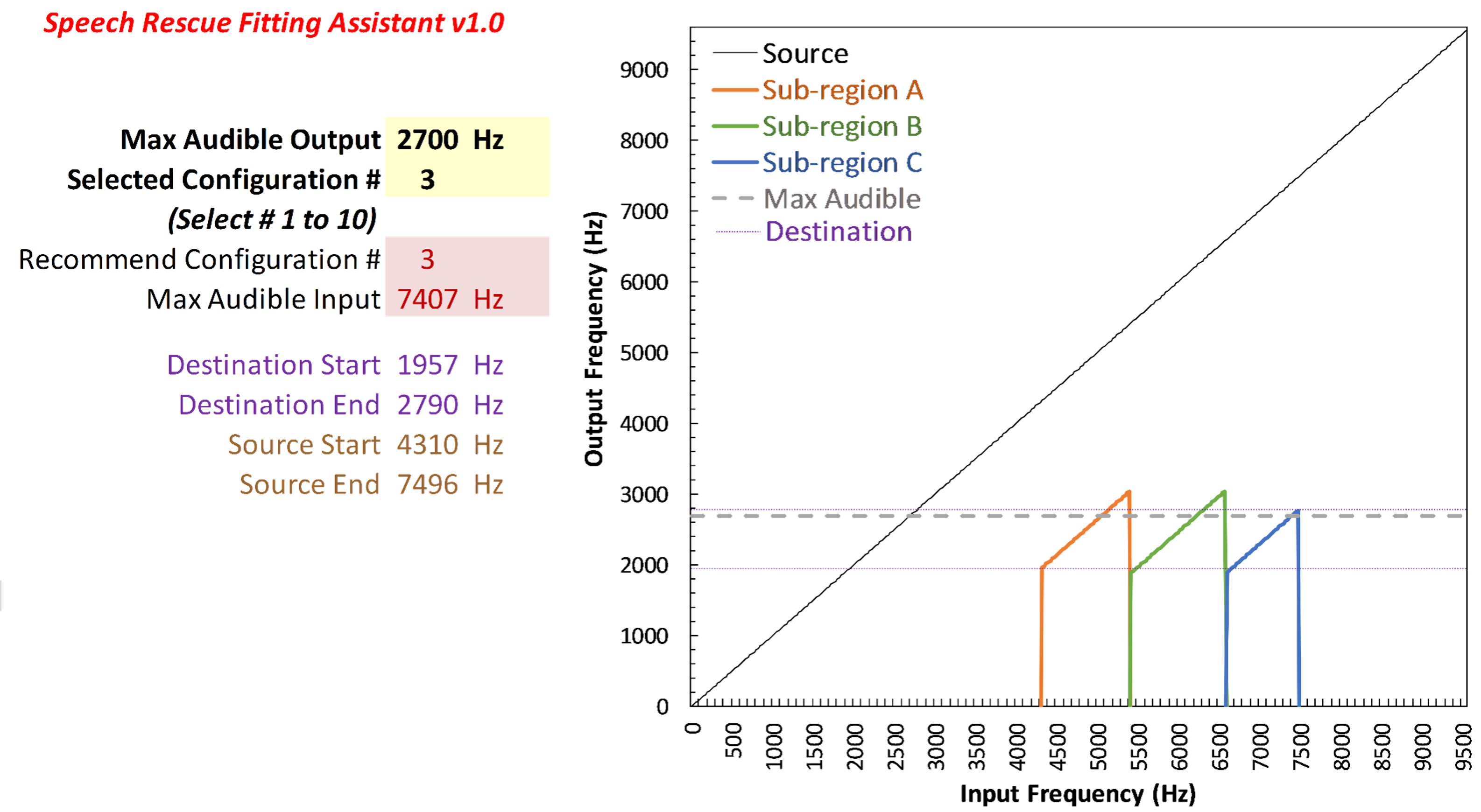
Figure 38. Visualization of the Speech Rescue Fitting Assistant and manufacturer’s software for a hearing aid configuration with a Maximum Audible Output Frequency (MAOF) of 2700 Hz. Upon entering this MAOF in the yellow box, the software recommends configuration number 3, as indicated in the red box. This configuration divides the input spectrum into three sub-bands. Each sub-band undergoes linear transposition and is overlaid in the output.

Shown in Figure 38 is how the second example would appear on the Fitting Assistant and manufacturer’s software. Again, the maximum audible output frequency at 2700 Hz is entered into the yellow box, which tells us in the red box that the recommended configuration is number 3. This time, notice how the input spectrum is divided into three sub-bands, each linearly transposed and overlayed in the output.

Phonak (Original) Frequency Lowering

Part VII reviews Phonak’s original Soundrecover algorithm. Phonak was the first of three manufacturers to implement nonlinear frequency compression. The original version of SoundRecover was in Phonak products from 2008 to 2016. Information about this algorithm is valuable because there are some generalities among the different varieties of nonlinear frequency compression and because Phonak’s latest version of frequency lowering, SoundRecover2, is a variation of this method.

Frequency Lowering Method

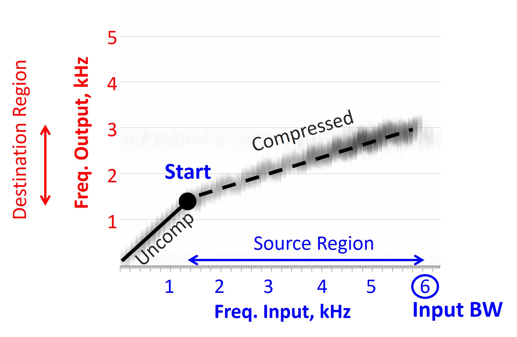
Figure 39. Spectrogram displaying the output of a hearing aid employing the SoundRecover algorithm during a continuous frequency sweep. The x-axis shows the instantaneous frequency of the input signal from a loudspeaker, while the y-axis represents the frequency emitted from the hearing aid receiver. This algorithm splits the incoming audio spectrum at a start frequency of 1.5 kHz, with frequencies below this threshold remaining uncompressed and outputted at their original frequencies. Frequencies above 1.5 kHz undergo compression with a ratio of 1.9 to 1 in this case, resulting in frequency lowering. The input bandwidth for compression in this example ranges from 1.5 kHz to 6 kHz, resulting in an output destination region spanning from 1.5 kHz to 3 kHz.

Figure 39 shows a spectrogram of a continuous frequency sweep as recorded from a hearing aid with SoundRecover. The x-axis corresponds to the instantaneous frequency of the signal being played from a loudspeaker, and the y-axis corresponds to the frequency of the signal coming from the hearing aid receiver. All nonlinear frequency compression algorithms divide the incoming spectrum into two parts at the start frequency, which is 1.5 kHz in this example. Everything below the start frequency is uncompressed. That is, sounds coming into the hearing aid at these frequencies come out at the same frequencies. It is called the start frequency because sounds above this frequency are compressed. The amount of frequency lowering is then determined by the compression ratio, which is 1.9 to 1 in this example. Later, it will be explained how the “compression ratio” is defined differently by the manufacturers. Still, one thing they have in common is that higher compression ratios result in more frequency lowering. In this example, the source region for compression spans from 1.5 kHz to 6 kHz in the input, making the input bandwidth 6 kHz; this is the highest frequency represented by the output. In this example, the destination region of the output is from 1.5 to 3 kHz. Finally, with the Phonak algorithm, the clinician controls frequency lowering by choosing different combinations of parameters for the start frequency and the compression ratio. The clinician can manipulate these parameters independently or choose a preset combination from a small set created by the programming software specifically for the hearing aid user’s audiogram.

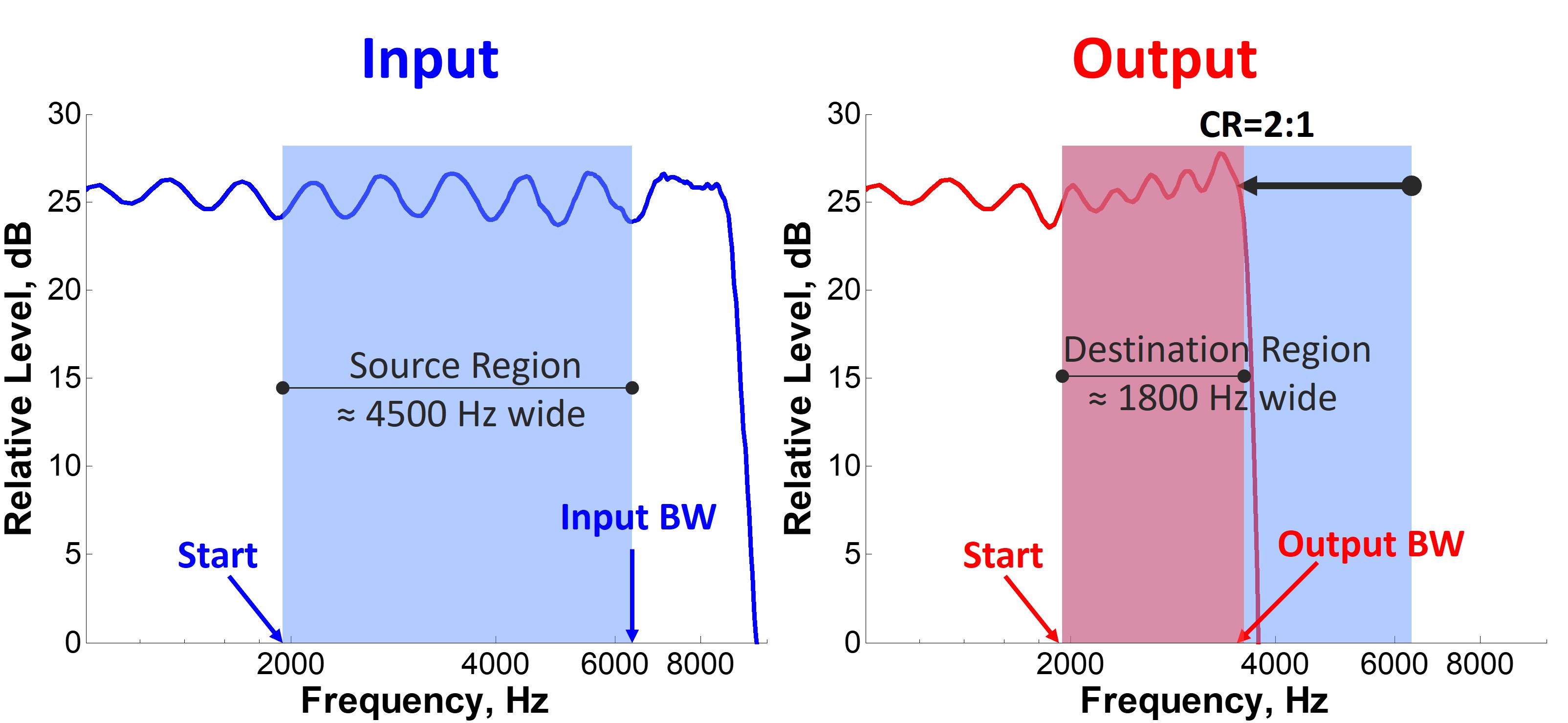
Figure 40. Side-by-side comparison of sound spectra before and after processing through a nonlinear frequency compression algorithm. The left figure displays the spectrum of the original input sound, characterized by a spectral ripple with regular frequency intervals between peaks and valleys. This source band starts at 1800 Hz and extends to 6300 Hz, covering a bandwidth of 4500 Hz. The right figure illustrates the transformed spectrum post-frequency lowering. Notable observations include the preservation of the ripple frequency spacing below the start frequency of 1800 Hz, indicating no compression in this range. Above the start frequency, however, the ripple spacing becomes compressed, akin to a condensed spring, resulting in a tighter frequency distribution in the output.

Figure 40 illustrates how nonlinear frequency compression algorithms work. The figure on the left is the spectrum of an actual input sound to one of these algorithms. It has a spectral ripple, meaning it has regular frequency spacings between its peaks and valleys to more easily observe what happens in the output after frequency lowering. In this example, the source region started at 1800 Hz and extended for another 4500 Hz, putting the input bandwidth at 6300 Hz. The figure on the right shows the signal spectrum after frequency lowering. First, notice how the frequency spacing of the ripples is maintained below the start frequency. Next, notice how the frequency spacing is condensed above the start frequency like a spring so that the same number of ripples encompasses a smaller frequency range in the output.

What Does “Nonlinear” Mean?

The discussion up to this point begs the question of what it really means to be nonlinear. If you ask an engineer, they will probably tell you that all compression is nonlinear by definition. However, the field uses the term “nonlinear” to refer to the generic concept that the frequency space is divided into two parts at a given start frequency so that only frequencies above it are altered. Phonak may have introduced the term “nonlinear frequency compression” to distinguish their revolutionary form of frequency lowering from earlier forms of frequency compression that operated throughout the entire frequency range, down to the very lowest frequency.

The manufacturers use different terms for what I have identified as the start frequency. Other terms include “cut-off frequency” and “f_min,” referring to the minimum frequency subjected to lowering. But they all refer to the same concept. Furthermore, they use the term compression ratio to define how frequencies at the hearing aid input are remapped in the output. For all of them, higher compression ratios correspond to a greater reduction or squeezing of the source bandwidth. However, it is critically important to understand that the relationship between input and output differs by manufacturer. For the Sonova (Phonak and Unitron) products, the mathematical expression that defines the relationship between the input and output frequencies really does require a nonlinear equation so that the frequency relationship ends up being linear on a log scale. In contrast, with ReSound, the relationship between the input and output frequencies is linear above the start frequency, so it can be considered a frequency divider. Finally, with Signia, after carefully documenting the output of every possible setting they offer in their software, I still have yet to determine the precise mathematical relationship between the input and output frequencies.

This discussion boils down to the major teaching point that while all of these manufacturers use the term compression ratio to refer more or less to the same concept, the value reported for compression ratio is incompatible across manufacturers. So, if you switch a hearing aid user from one brand to another, you cannot simply copy the settings and expect the same outcome. This reinforces one of the main points in Part I: when using frequency lowering, at minimum, you must know what the manufacturer is doing underneath the hood and verify the output of your fittings.

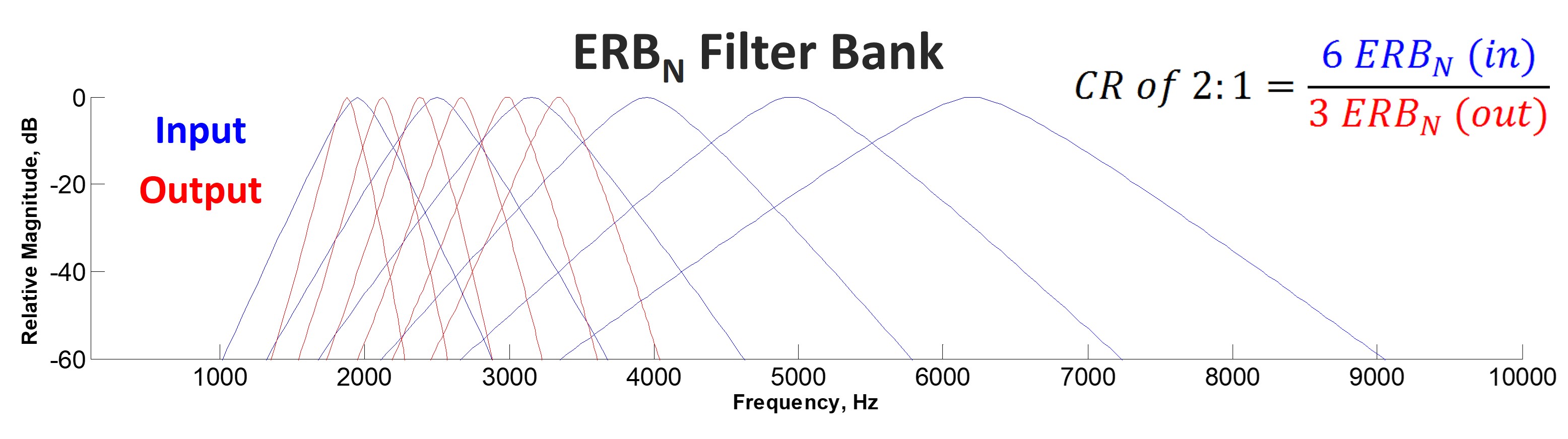
Figure 41. Illustration of the compression ratio concept in Phonak’s SoundRecover algorithm explained using the ERB (equivalent rectangular bandwidth) scale. This figure uses blue lines to represent how auditory filters on the basilar membrane process sound after compression. In the input (pre-compression), a sound that spans six auditory filters (as shown by red lines) is compressed so that it covers only three filters in the output (blue lines). This compression effectively means that each output auditory filter now encodes information that originally spanned two input filters, demonstrating a compression ratio of two-to-one. This visual representation helps to conceptualize the non-linear nature of Phonak's compression algorithm, emphasizing the focus on psychophysical rather than purely frequency-based scaling.

The compression ratio with the Phonak algorithm is not a simple linear division of input divided by output frequencies on a Hz scale. Instead, it closely corresponds to bandwidth reduction on a psychophysical scale. One such scale is the ERB scale, which stands for “equivalent rectangular bandwidth.” One ERB represents the filter properties of an auditory filter on the basilar membrane. The compression ratio reported by the original SoundRecover, more or less, corresponds to the number of auditory filters represented by the input compression band (CB) divided by the number of auditory filters represented by the output compression band. To illustrate this concept, the blue lines in Figure 41 show how an incoming sound that would normally span six of these auditory filters in the input will span only three in the output. After compression, one blue auditory filter encodes sounds that previously spanned two filters shown in red, yielding a compression ratio of two to one.

Demonstration of Algorithm Behavior

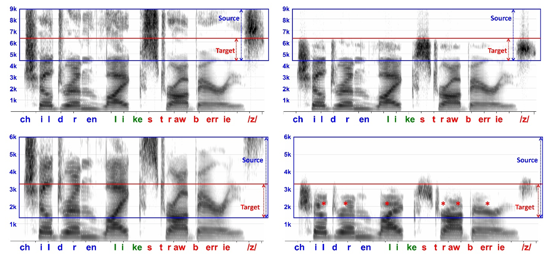
Figure 42. Comparative spectrogram analysis demonstrating the application of Phonak’s SoundRecover algorithm for different levels of high-frequency hearing loss, using the sentence from Figure 4. In the top panels with settings intended for mild-to-moderate high-frequency hearing loss, the source band ranges from 4.5 to 9 kHz (blue boxes). The top-right panel reveals the effect of SoundRecover: fricative sounds are compressed to around 6.3 kHz, while frequencies below the start frequency of 4.5 kHz remain unaltered, preserving the spectrum’s lower part. The bottom panels, with settings intended for moderate to severe high-frequency hearing loss, have a source band from 1.5 to 6 kHz (blue boxes). In the bottom-right panel, SoundRecover’s impact extends beyond frication, also compressing the second and third formants and their transitions as indicated by the red asterisks.

The panels on the left of Figure 42 show the spectrogram of the same sentence used in Figure 4, which demonstrated the limitations of limited high-frequency audibility. Here, they are used to demonstrate the behavior of the SoundRecover algorithm. In all panels, the blue boxes indicate the source region, and the red boxes indicate the target or destination region. The top panels show how the algorithm might be used for individuals with mild-to-moderate high-frequency hearing loss, with the source band extending from 4.5 to 9 kHz. Compared to the top-left panel, the top-right panel shows that the only speech sounds affected are those with frication, which is squeezed down to around 6.3 kHz. Notice how the spectrum below the start frequency, 4.5 kHz, is preserved.

The bottom panels show how the algorithm might be used for individuals with moderate to severe high-frequency hearing loss, with the source band extending from 1.5 to 6 kHz. Compared to the bottom-left panel, the red asterisks in the bottom-right panel shows how the second and third formants and formant transitions are reduced in addition to the frication. Refer to Part I, specifically Figure 6, for how this might negatively affect speech perception.

Programming Software Settings

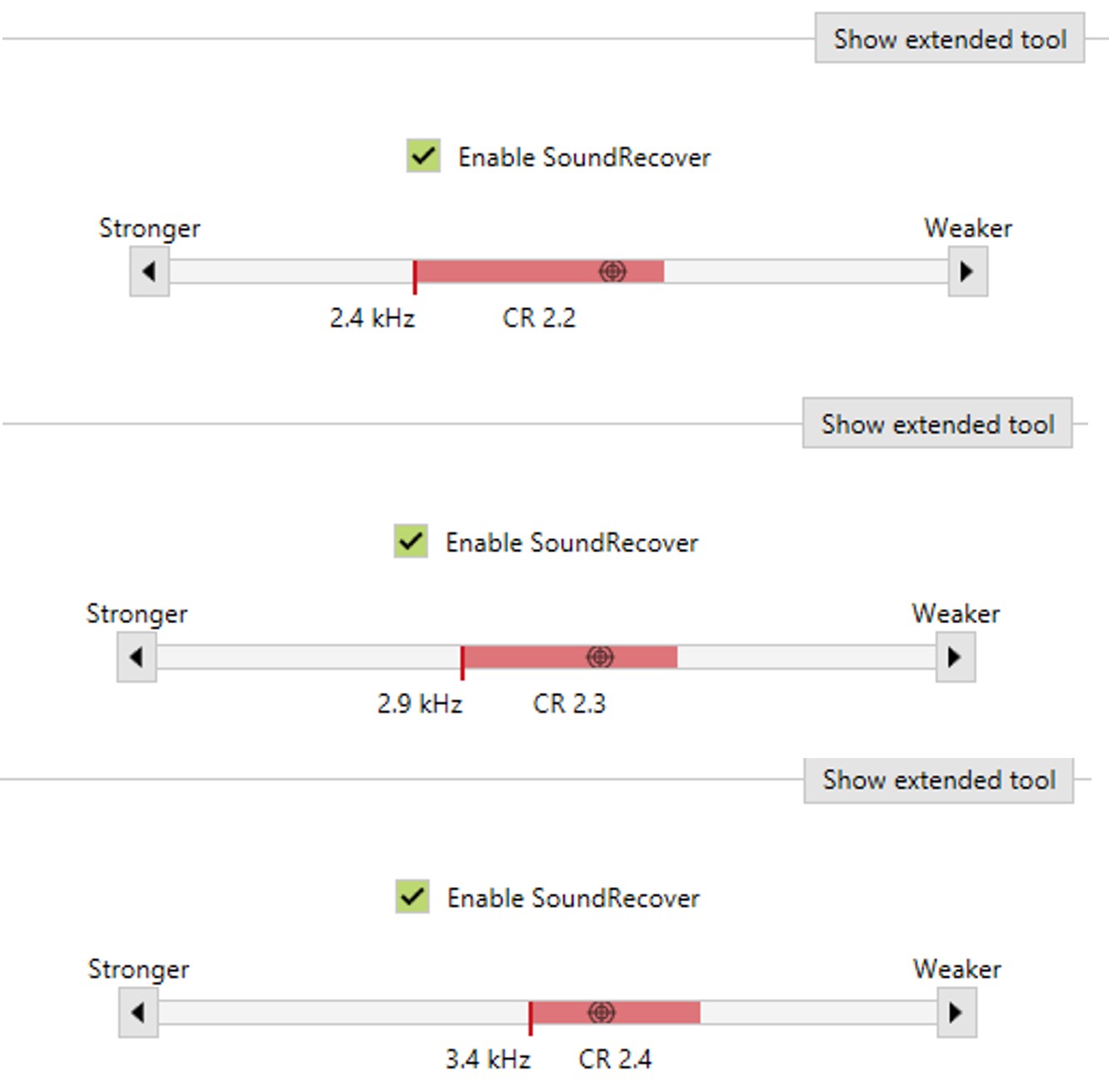
Figure 43. Display of preset start frequency and compression ratio settings in Phonak’s Target 9.0 software. The top panel shows stronger frequency lowering settings, achieved by moving the slider to the left, resulting in lower start frequencies and higher compression ratios. Conversely, moving the slider to the right (middle and bottom panels) increases the start frequency and reduces the compression ratio, indicative of weaker frequency lowering settings. Additionally, the "Show extended tool" button provides the option to manually adjust the start frequency and compression ratio independently, offering further customization beyond the preset options.

Figure 43 shows preset start frequency and compression ratio combinations as they appear in the Target 9.0 software for the first example audiogram discussed below. The settings are changed by moving the slider to the left for stronger frequency lowering, which would entail lower start frequencies and higher compression ratios (top panel). As the slider is moved to the right, the start frequency increases and the compression ratio decreases, corresponding to weaker settings (middle and bottom panels). As with the other manufacturers, the process is a trial and error; you try a few settings, see what you get, and then try to bracket around an optimal setting. If you do not want to use the preset options, you can select the “Show extended tool” button, and you will be able to set the start frequency independently from the compression ratio. However, for the sake of example and to constrain our options, I will stick with the preset options.

Fitting Assistant: Goals

The fitting assistant for the original SoundRecover was my first fitting assistant for frequency lowering. In fact, it was during the development of the SoundRecover fitting assistant in early 2009 that the concept and term Maximum Audible Output Frequency (MAOF) was coined. As the Phonak changed their algorithm over the years, I introduced different versions of the SoundRecover fitting assistant. The last version is the third one, version C. It was used with the Venture platform, which was last produced in 2016.

The goal behind the SoundRecover fitting assistant is to maximize the use of the audible bandwidth. The fitting assistant uses a fuzzy logic model that weights four variables to select the optimal setting that meets this goal. The first variable is the audible output bandwidth, defined as the highest frequency in the amplified output that is audible after frequency lowering. The goal is to choose a setting where this frequency is reasonably close to the Maximum Audible Output Frequency, which, if you recall, is determined with frequency lowering deactivated. The input frequency corresponding to this output frequency defines the audible input bandwidth: it tells how much of the source signal is made audible by frequency lowering. Within certain limits that I will discuss in more detail, generally, the higher this is, the better. The next variable is the start frequency. Generally, a higher start frequency is better because it will have fewer adverse effects on the formants. And then, everything else being equal, a lower compression ratio is favored over a higher compression ratio to help preserve the frequency resolution of the sounds coming out of the hearing aid.

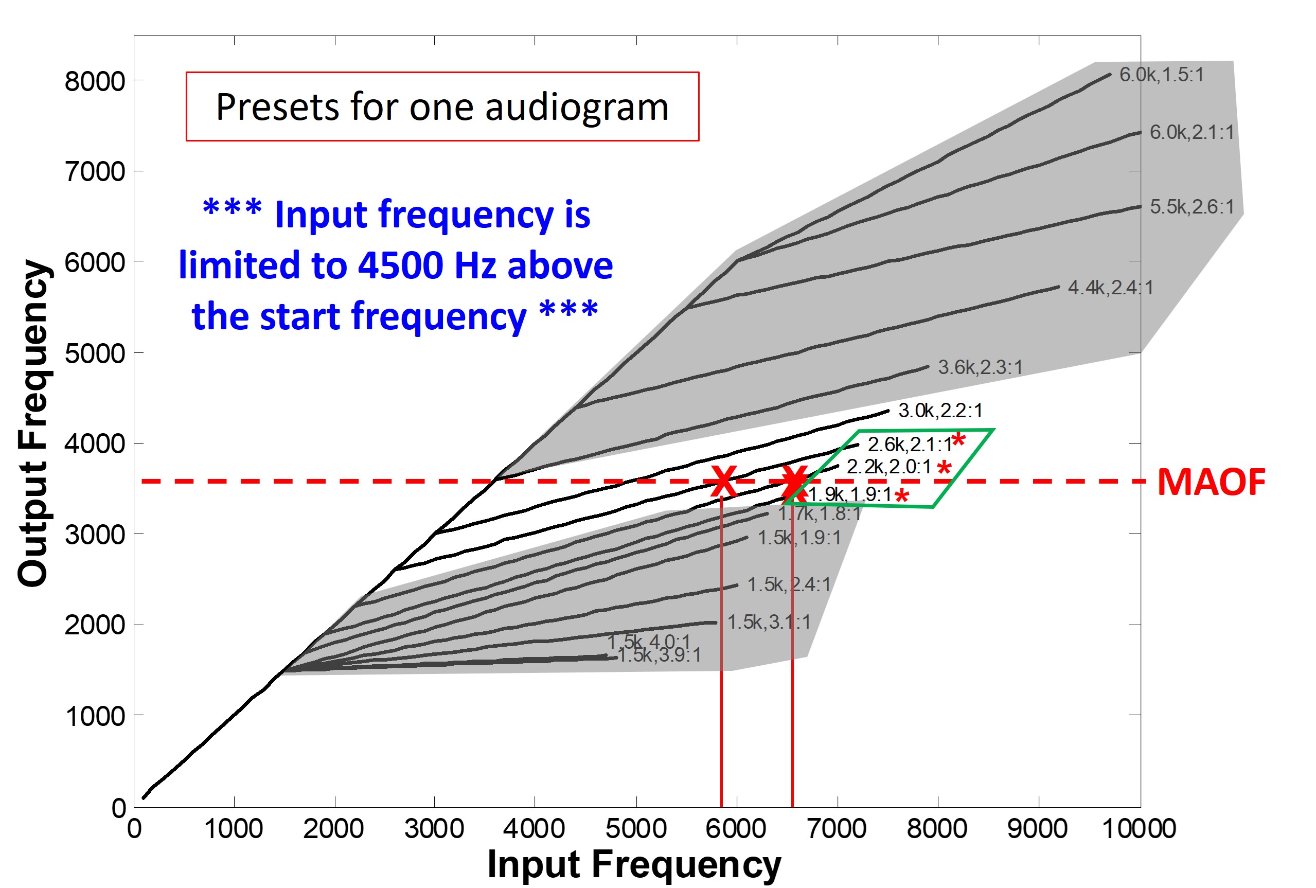
Figure 44. Visualization of input-output curves for preset SoundRecover settings based on a specific audiogram, with each setting characterized by a start frequency (in kHz) and a compression ratio. Each curve is capped at 4500 Hz above its start frequency, a constraint rooted in Phonak’s original SoundRecover design and retained in the fitting assistant to prevent excessive frequency lowering. The key element in this figure is the Maximum Audible Output Frequency (MAOF), marked by a red dotted line. This line represents the upper limit of frequencies audible to the hearing aid user. Settings with start frequencies above the MAOF are ineffective for the user and are therefore grayed out, as are the most aggressive settings at the bottom to avoid excessive frequency lowering. The most-ideal settings are those where the maximum output frequency, indicated by red X's, aligns closely with the MAOF. These settings maximize the use of the user's audible bandwidth, ensuring that the frequency-lowered information remains within their hearing range.

Figure 44 shows a family of input-output curves you would obtain for one audiogram if you choose among the preset options when selecting the SoundRecover setting. Each setting is defined by the start frequency in kHz, followed by the compression ratio. It is important to note that each line is limited to 4500 Hz above the start frequency. This is the limit mentioned previously. The reason for this is that Phonak imposed this limit when they first released SoundRecover. When they removed this limit, it made sense to retain it for the fitting assistant because it helps constrain the fuzzy logic model from choosing too much frequency lowering (that is, very low start frequencies and/or high compression ratios) to maximize the input bandwidth. In other words, it helps balance the weight assigned to each variable and constrain the number of options under consideration.

The maximum audible output frequency, the MAOF, is the most important thing to pay attention to because it tells us how much of the cochlea we have to work. In the example shown in Figure 44, the MAOF is indicated by the red dotted line. For this example, we can immediately dismiss all the settings with start frequencies above the MAOF because the hearing aid user cannot hear any frequency-lowered information; hence, they are grayed out. We can also dismiss the settings at the bottom since we want to avoid too much frequency lowering; hence, they are also grayed out. Recall that these lines are artificially truncated below the MAOF for the reasons I mentioned earlier. Regardless, for the most aggressive settings at the bottom, the output bandwidth after frequency lowering will be less than what we had to start with, indicating that we will not have effectively used the hearing aid user’s audible bandwidth. From this perspective, we want to consider the settings whose maximum output frequency, as indicated by the red X’s, is close to the red dotted line. Shown are three candidate settings. We might eliminate the first setting (2.6 kHz start, 2.1:1 compression ratio) because the hearing aid user does not gain as much input bandwidth as the other two, which cross the x-axis at a higher frequency. Of the two remaining settings, we might choose the one with the higher start frequency (2.2 kHz vs. 1.9 kHz) to better preserve the low-frequency formants. This is the basic logic that guides the SoundRecover fitting assistant.

Fitting Assistant: Example 1

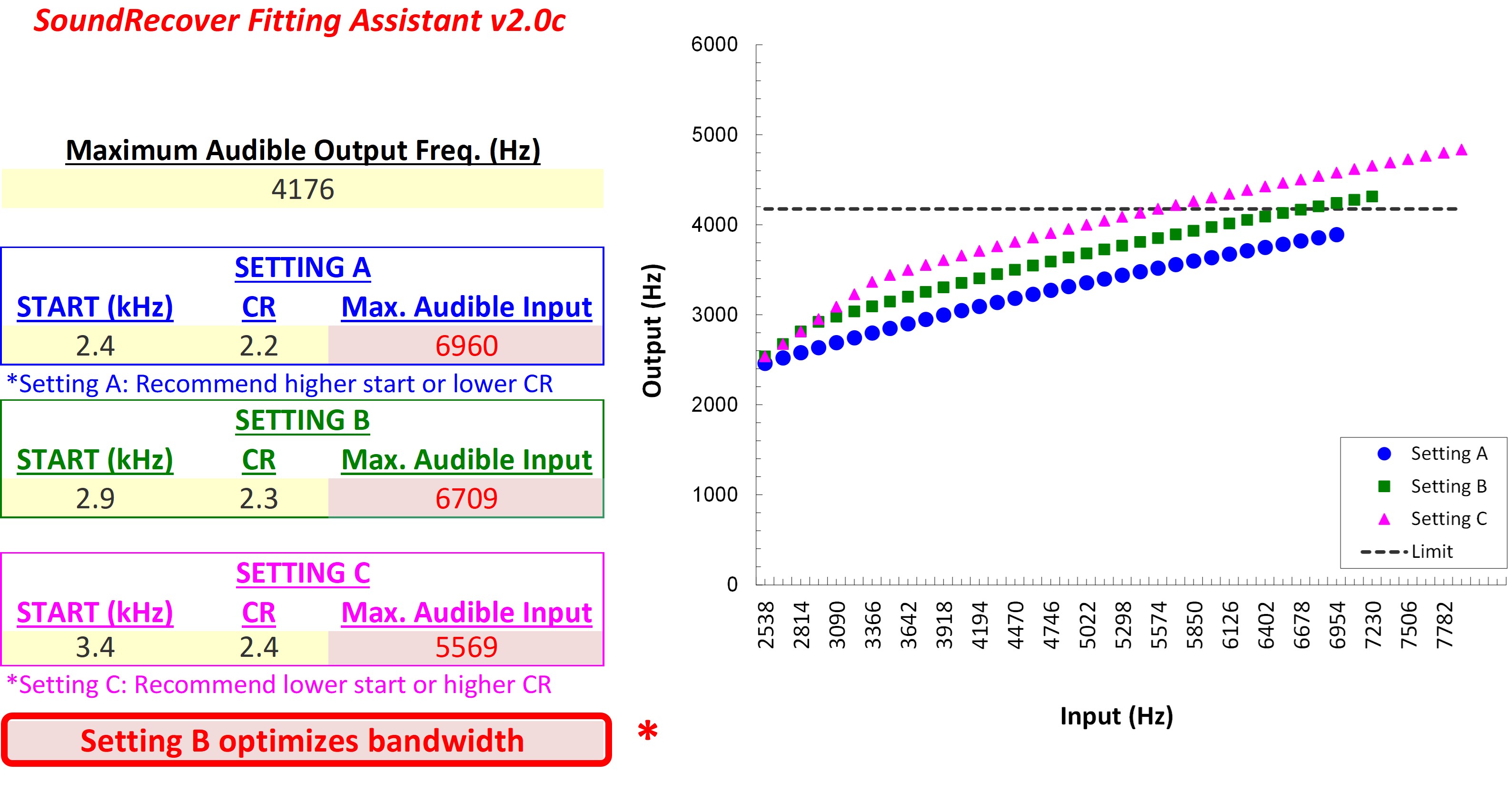
Figure 45. Display of the SoundRecover Fitting Assistant in action, demonstrating how it aids in fine-tuning frequency-lowering settings for an individual hearing aid user. The user's Maximum Audible Output Frequency (MAOF) of 4176 Hz is input at the top. Start frequencies and compression ratios for the three different settings (A, B, and C) from Figure 43 are entered, with the Fitting Assistant calculating the maximum audible input frequency for each setting, as indicated in red boxes.

Figure 45 demonstrates the use of the SoundRecover Fitting Assistant. The maximum audible output frequency of 4176 Hz was entered into the box at the top of the fitting assistant. The start frequency and compression ratio for the three settings shown in Figure 43 were entered into the boxes labeled Setting A, B, and C, respectively. For setting, the value in the red box reports the maximum audible input frequency, where on the x-axis, the input-output function crosses the MAOF. Notice that right below Setting A and Setting C, the fitting assistant makes specific recommendations for optimizing the settings based on the fuzzy logic model described earlier. Also, notice that there are no recommendations for Setting B and that the bottom box indicates that this one optimizes the bandwidth relative to the other settings. This is useful if you have two or more settings with no recommendations for changing the start frequency or compression ratio. Once you find a setting that you think will work, as illustrated here, it is good practice to try the next weakest setting on the slider and the next strongest setting on the slider to be sure that you have explored the range of options.

Fitting Assistant: Example 2

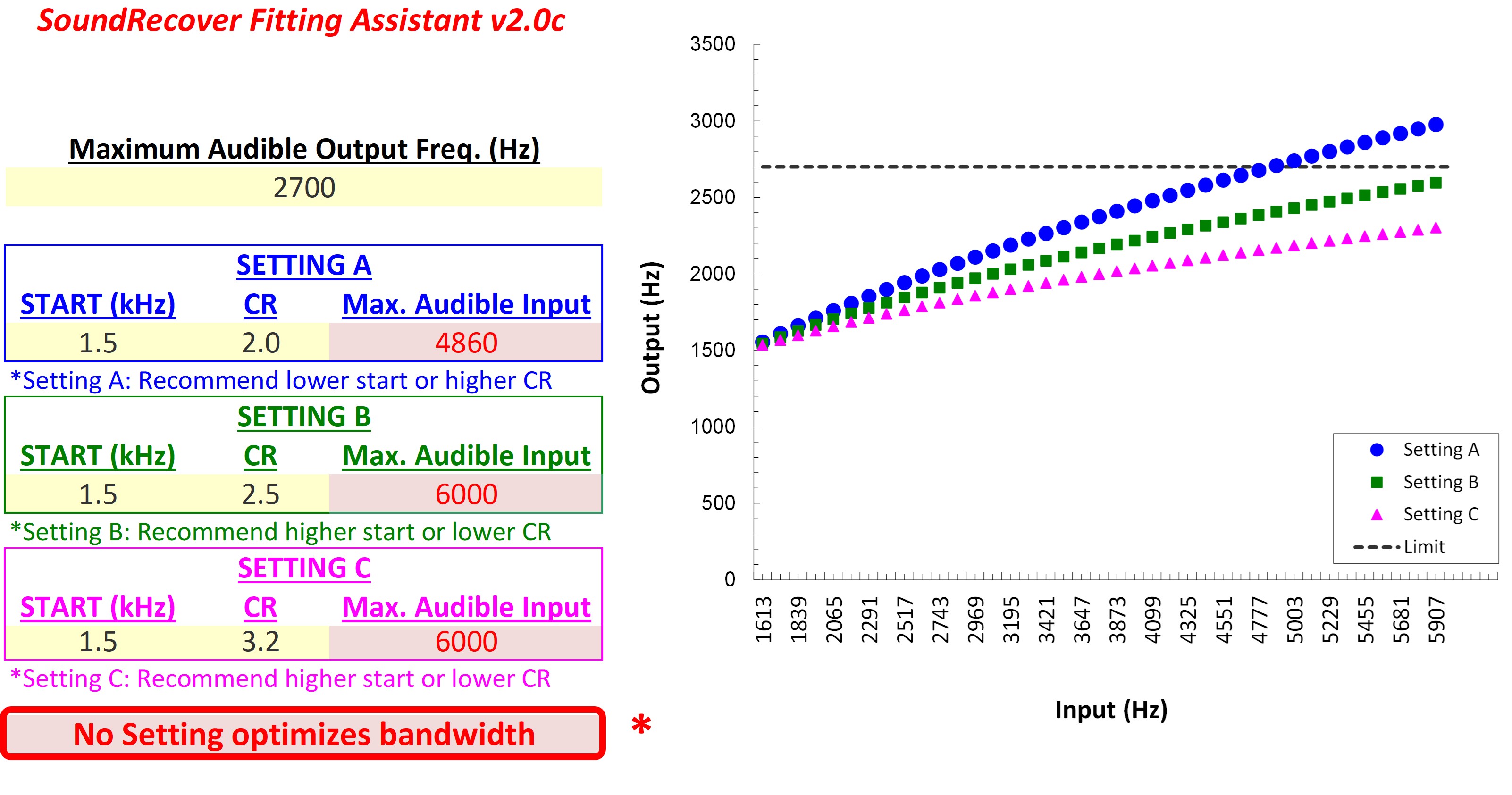
Figure 46. Visualization of the SoundRecover Fitting Assistant showcases the three best-preset options for an audiogram with a Maximum Audible Output Frequency (MAOF) of 2700 Hz. Notably, the final recommendation in the red box at the bottom reveals that none of these three settings optimally maximizes the bandwidth per the criteria established by the fuzzy logic model.

Figure 46 shows SoundRecover Fitting Assistant with the three best-preset options I found when I entered the audiogram into the Phonak software for the second example used throughout, which had a maximum audible output frequency of 2700 Hz. For Setting A, the fitting assistant recommended a lower start frequency or higher compression ratio, in other words, a stronger setting. However, the lowest start frequency available is 1.5 kHz, so the only option when I moved the slider to the left was a 1.5 kHz start frequency with a 2.5 to 1 compression ratio. Interestingly, the fitting assistant recommended a weaker setting, but there was nothing between what I entered for Setting A and Setting B. For completeness, I entered the next strongest setting for Setting C, which increased the compression ratio to 3.2 to 1. Notice, then, that the final recommendation in the red box at the bottom indicates that none of the three settings optimizes bandwidth according to the rules set by the fuzzy logic model. If I had to, I would choose Setting B because it has the same maximum audible input frequency as Setting C but uses a lower compression ratio.

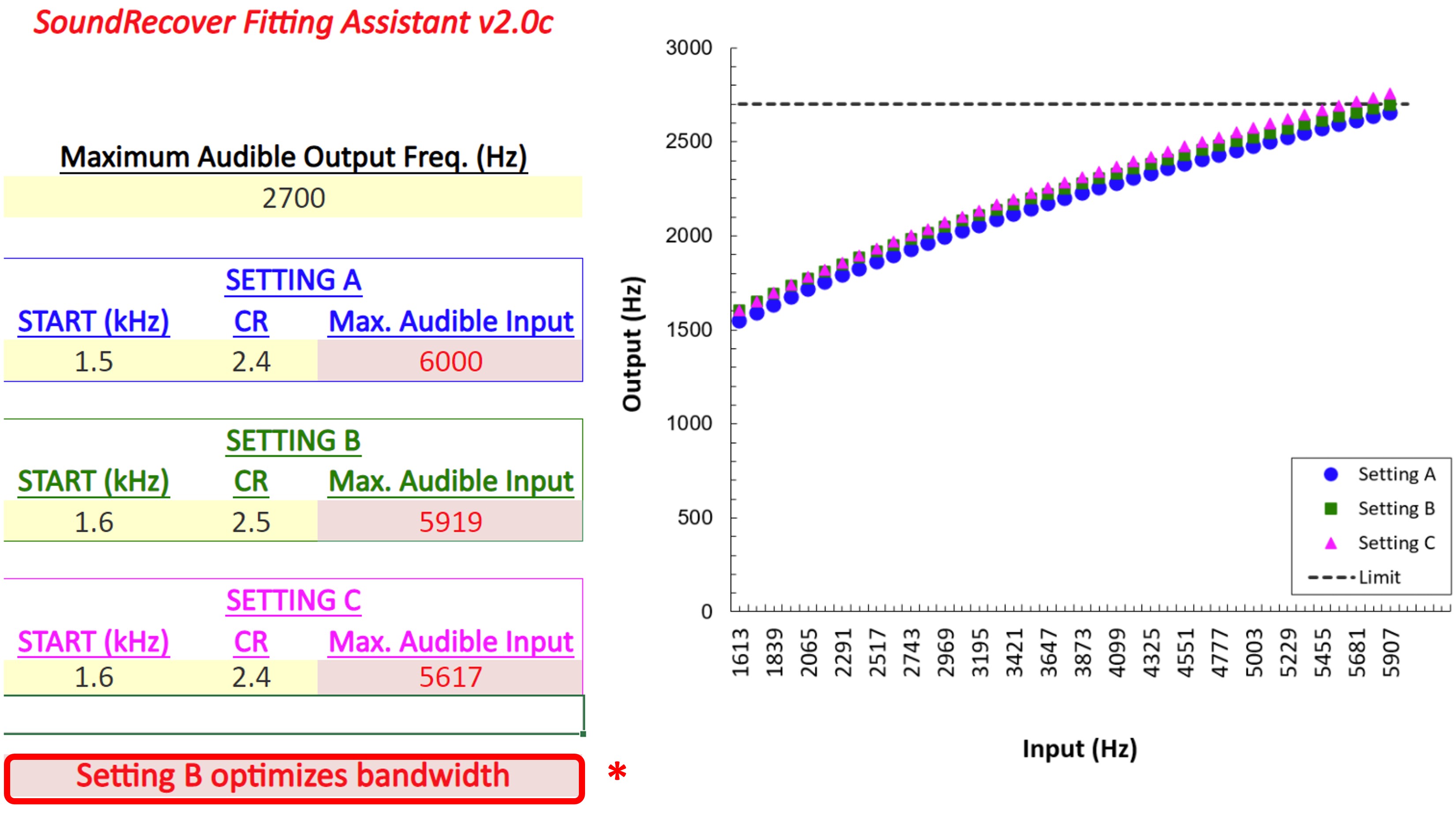
Figure 47. Representation of adjustments made using the “Show extended tool” feature in Phonak’s programming software, following the observation that none of the presets in Figure 46 optimized bandwidth as per the established criteria. Modifications were applied to the original Setting B from Figure 46, which had a start frequency of 1.5 kHz and a compression ratio of 2.5 to 1. Unlike the previous scenario, the Fitting Assistant now does not suggest further modifications to these settings; it identifies Setting B, with its adjusted start frequency and maintained compression ratio, as the best option among the three.

Considering that none of the preset options optimized bandwidth according to our rules, I went into the programming software using the “Show extended tool” button. Then, I made slight manipulations to Setting B in Figure 46, which had a 1.5 kHz start frequency and a 2.5 to 1 compression ratio. As shown in Figure 47, I kept the start frequency the same for Setting A and decreased the compression ratio to 2.4 to 1. I increased the start frequency to 1.6 kHz for Setting B but kept the compression ratio the same as before. For Setting C, I increased the start frequency and the compression ratio. Now, we have the opposite situation as the previous slide because the fitting assistant does not recommend any changes for the three settings. However, it indicates that the best of the three corresponds to the values entered for Setting B.

Signia Frequency Lowering

Part VIII discusses nonlinear frequency compression in the Signia hearing aid products.

Frequency Lowering Method, Demonstration of Algorithm Behavior, and Programming Software Settings

Figure 48. Graphical representation of the frequency input-output function for a Signia hearing aid, accompanied by a screenshot from the Signia Connexx 9.11 programming software. The x-axis depicts the input frequencies to the hearing aid, with the source region extending from the minimum frequency (f_min) to the end frequency (fend), which is fixed at 11.5 kHz for these devices. The y-axis shows the corresponding output frequencies after processing. In Signia’s system, f_min functions similarly to the start frequency in Phonak and ReSound aids, marking the threshold above which sounds are subjected to frequency lowering. Below f_min, sounds retain their original frequency in the output. f_max represents the highest output frequency corresponding to fend. The distance between f_min and f_max determines the compression ratio; a smaller gap results in a higher compression ratio.

Figure 48 shows a recording from one of the Signia devices and its frequency input-output function. The frequencies on the x-axis represent the sounds going into the hearing aid. The source region spans an area on the x-axis from f_min to fend. These are the two settings available to the clinician when programming Signia’s frequency lowering as indicated by the screenshot from the Signia Connexx 9.11 programming software at the top of the figure. fend is the maximum input frequency and is the same as what I have referred to in other parts as the input bandwidth, which is always 11.5 kHz for these devices. f_min is the same as the start frequency in the Phonak and ReSound hearing aids, whereby sounds below it come out at the same frequency as they come in. Sounds above f_min are subjected to lowering. The frequencies on the y-axis represent where each input frequency comes out of the hearing aid. f_min also serves as the anchor for the destination region. f_max is the output frequency corresponding to fend. As shown above, frequency compression in the Signia hearing aids is controlled by selecting f_min and f_max in 250-Hz steps on a slider. The amount of frequency compression — or the compression ratio — is determined by the spacing between these two controls: the closer they are, the higher the compression ratio.

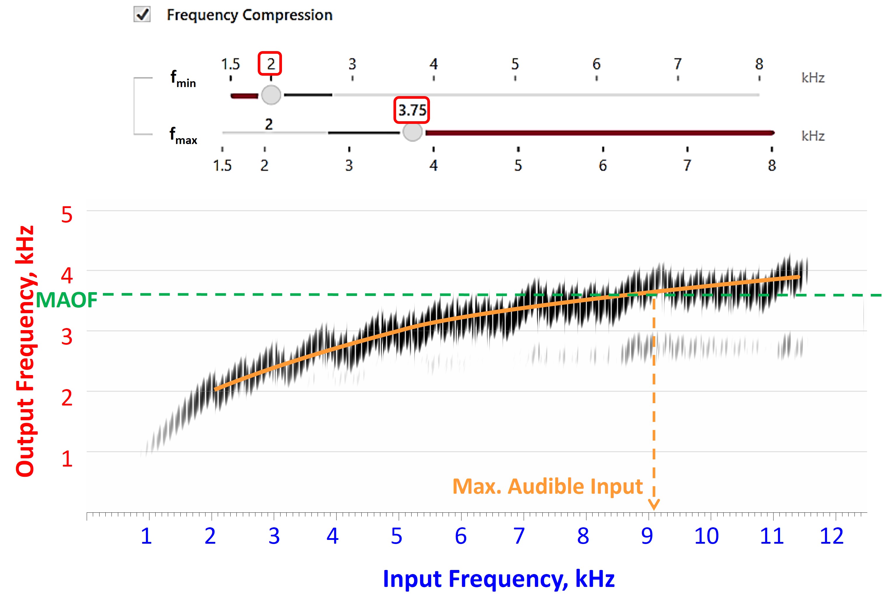
Figure 49. Same as Figure 48, but with a higher f_max. While a f_max greater than the MAOF corresponds to a smaller audible bandwidth, the lowered speech information may be more discriminable for the hearing aid user.

Hypothetically, if the maximum audible output frequency is 3.7 kHz, the output will have sounds represented up to 11.5 kHz from the input. If you believe more is better, this would seem reasonable. However, I argue that choosing a slightly higher f_max is better. While a portion of the source signal will be put in the destination region where the hearing aid user cannot hear it, the tradeoff is that there will be less compression. The idea is that this may be better for perception by making better use of the frequency-lowered signal. Therefore, increasing f_max one setting higher will cause the yellow line representing the frequency input-output function to intersect with the maximum audible output frequency at an input frequency of around 9 kHz. My fitting assistant will report this value.

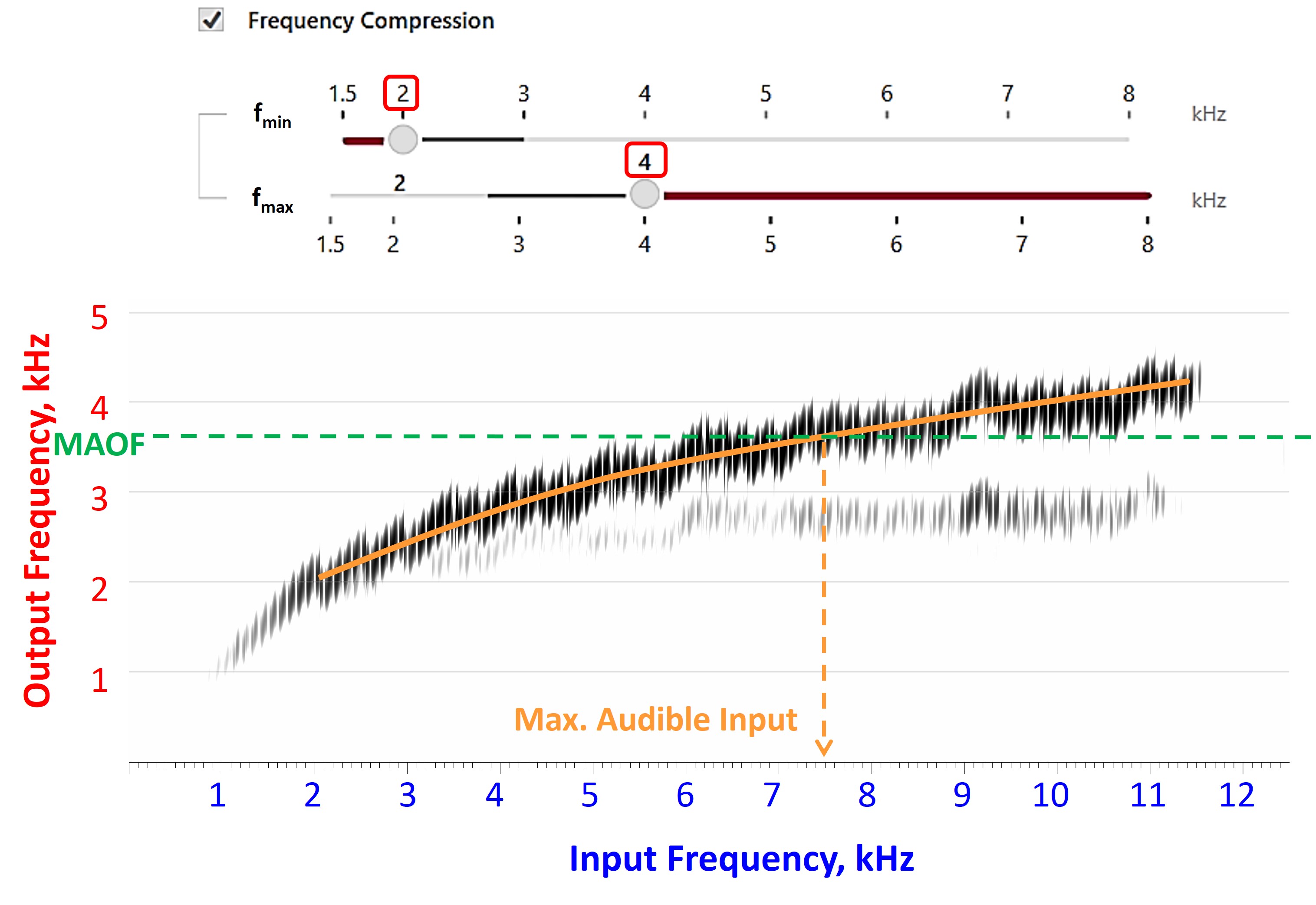
Figure 50. Same as Figures 48 and 49, but with an even higher f_max.

You might consider increasing f_max even higher, which would be 4 kHz. More of the frequency-lowered sound will be put in a region beyond audibility for the hearing aid user to access information out to about 7.5 kHz. Compared to the previous setting, where we achieved audibility for input sounds up to 9 kHz, this setting may be less optimal. Or, if you consider that this setting may result in a better quality signal because it has less compression, then it may be the better of the two.

Fitting Assistant: Goals

I have a few guidelines to help you choose between the frequency-lowering settings in the Signia devices. These guidelines will not titrate to one particular setting. Instead, the idea is to establish first principles that hopefully prevent adverse outcomes. Further research is needed to establish which of the remaining settings is best.

1. The first priority is to ensure that f_max — the highest output frequency — is at least as high as the maximum audible output frequency. I have established this principle the other fitting assistants. The idea is to make the most effective use of the hearing aid user’s audible range; you cannot do this if you restrict their aided bandwidth by implementing frequency lowering that is too aggressive. Again, remember to watch the compression ratios. As I just discussed, do not be afraid to set f_max beyond the maximum audible output frequency. Considering you can control f_max in 250-Hz increments, I recommend 1 or 2 settings higher than the maximum audible output frequency. While it might seem ideal to match f_max to the MAOF as closely as possible since the hearing aid user will have access to sound beyond 11 kHz, this is likely overkill since it will result in too much compression. Even though the hearing aid user will have less access to high-frequency sounds, they may be able to use the frequency-lowered sound more effectively.
2. The second priority is based on the principle that adverse outcomes are more likely when the first two formants of speech are altered. Therefore, the priority is to start frequency lowering above 2.25 kHz if possible since this is out of the range of most second-formant frequencies in English. This recommendation is based on research I did with a simulation of the Phonak version of this algorithm, where we observed detriments to many vowels and some consonants with start frequencies lower than this frequency. On the other hand, once the start frequency was around 2.25 kHz or higher, we did not observe any adverse side effects.
3. The third priority directly refers to the amount of compression or the compression ratio. Specifically, it refers to the frequency range of the audible destination region, which is bounded by the f_min and the maximum audible output frequency. Therefore, I recommend keeping this range between 1.25 and 2.0 kHz. If it is less than this, you probably have too much compression. If it is greater than this, you are better off increasing f_min to protect the formant frequencies.

It should be noted that the Connexx software will not allow you to set f_min and f_max less than 0.75 kHz of each other, which you would not want to do anyway because of its effect on the amount of compression. Finally, with moderately-severe hearing losses, you might face a situation where you have to decide between setting f_min lower than 2.25 kHz and having a narrow audible destination region. Many times, this may be unavoidable. However, it is worth noting that my research indicates that the hearing aid user may still benefit from an audible destination region as narrow as 1 kHz if it means setting f_min at 2.25 kHz or higher.

Fitting Assistant: Example 1

To illustrate the frequency-lowering fitting assistant for Signia, I will use the first example, where the maximum audible output frequency was 4176 Hz. More or less, this is a trial-and-error approach where we try to abide by the priorities listed above.

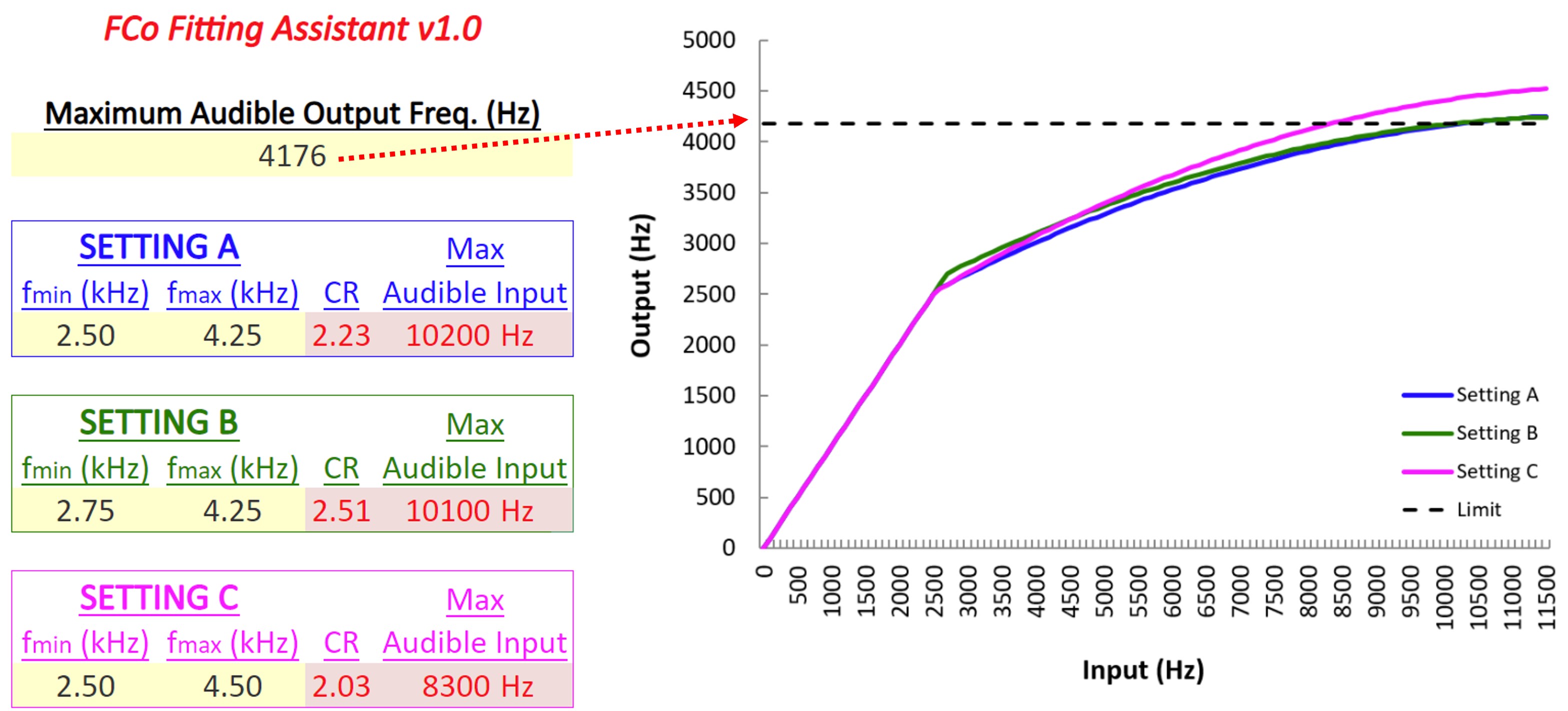
Figure 51. Screenshot of Signia’s fitting assistant displaying three potential frequency compression settings for the first example. Up to three combinations of f_min and f_max can be entered for comparison. For each entry, the compression ratio and maximum audible input frequency are reported. The MAOF is input at the top of the fitting assistant and represented on the graph by a black horizontal line.

Figure 51 shows a screenshot of the fitting assistant for Signia frequency compression with three candidate settings entered in the boxes on the left. All three settings have a f_max greater than or equal to the maximum audible output frequency. Furthermore, all three have a f_min greater than or equal to 2.25 kHz. Finally, they all have an audible destination region between 1.25 – 2.0 kHz. Therefore, all three of these are viable settings. As with the other fitting assistants, the maximum audible output frequency is entered into the box at the top, plotted as the black horizontal line on the graph. Recall that sounds above this line will be inaudible to the hearing aid user. The fitting assistant can help you make informed decisions based on several variables for your hearing aid user.

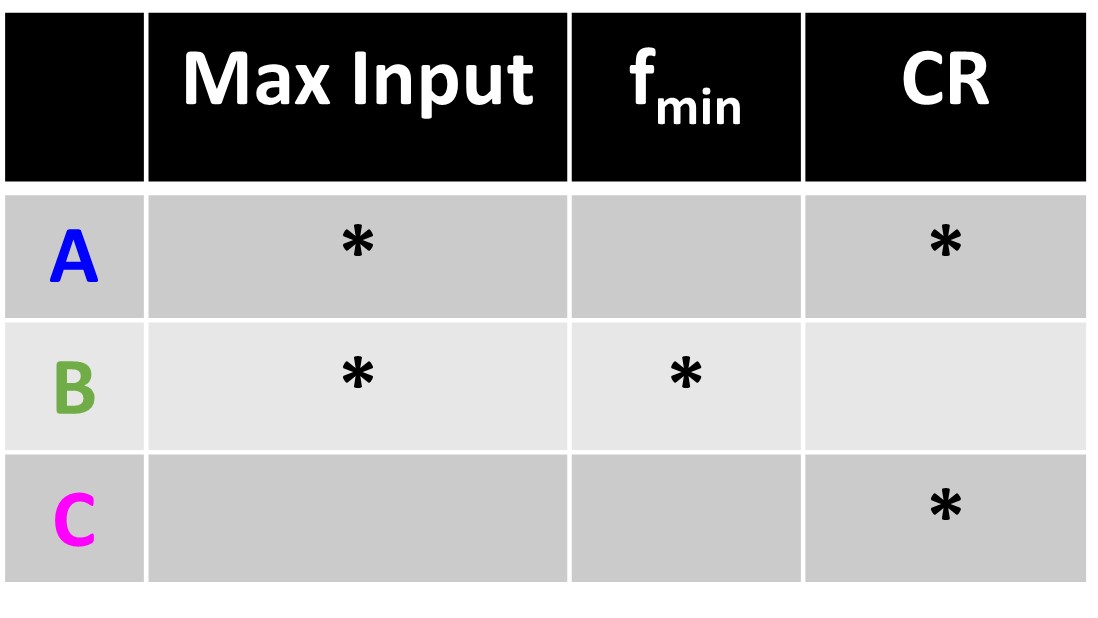
Table III. Comparative analysis of the three frequency compression settings shown in Figure 51, with asterisks indicating the more favorable aspects of each setting. In summary, Setting A is favorable for its lower compression ratio, Setting B for its higher f_min, and Setting C for its lower compression ratio despite a reduced maximum audible input frequency.

Table III shows how the three settings differ. The asterisks indicate which setting is more favorable than the others regarding the maximum audible input frequency, f_min, and compression ratio (CR). Settings A and B both have a high maximum audible input frequency; however, setting A has a lower or more favorable compression ratio, while setting B has a higher or more favorable f_min. Finally, while setting C has a much lower maximum audible input frequency than the others, it has the lowest compression ratio; recall that a greater maximum audible input frequency is not necessarily better. Unfortunately, there is no research data to tell us which hearing aid users will do best with each of these three settings or if they will all lead to similar outcomes. The overall goal is to help ensure you do no harm with frequency lowering by making speech perception worse than with it deactivated.

Fitting Assistant: Example 2

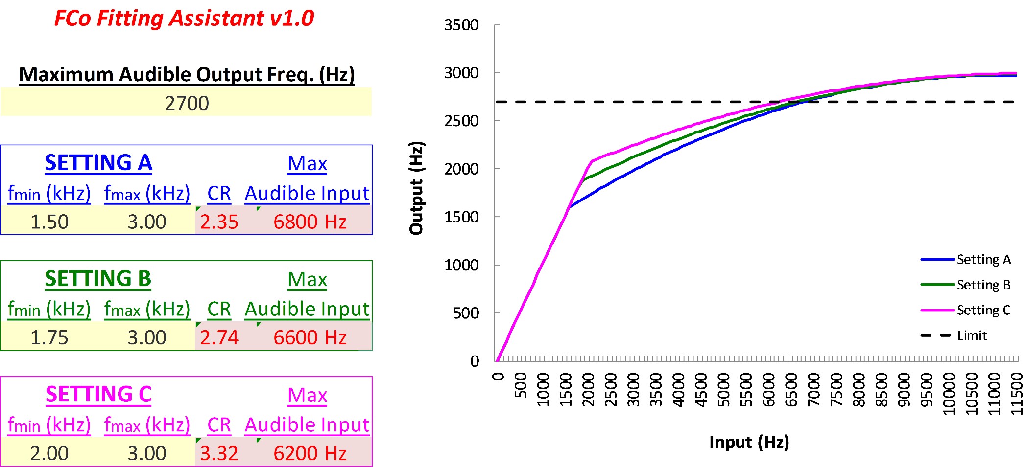
Figure 52. Screenshot of Signia’s fitting assistant displaying three potential frequency compression settings for the second example.

The second example, as shown in Figure 52, has fewer options because the maximum audible output frequency is only 2700 Hz. For each of these settings, I put f_max at 3 kHz because if I selected the next highest setting, 3.25 kHz, the maximum audible input would only be around 5.5 kHz, which might not provide the hearing aid user with as much high-frequency information. Furthermore, f_min needed to be less than 2.25 kHz to avoid compression ratios that were too high. Thus, there are only three possible settings for this hearing loss, which differ only in the setting for f_min. Perhaps, a sensible approach would be to try setting B because setting C has a high compression ratio, and setting A may affect more of the formant frequencies due to its lower f_min. But, again, the necessary research to help us make more definitive recommendations is lacking.

ReSound Frequency Lowering

Part IV provides a review of ReSound’s method of frequency lowering. They are the third manufacturer that offers a form of non-linear frequency compression called Sound Shaper.

Frequency Lowering Method

Frequency compression in ReSound’s products is linear or proportional. This means you can easily compute the output frequency by dividing the difference between the input and start frequencies by the compression ratio. For example, with a compression ratio of 2.0, if the input frequency is 1000 Hz above the start frequency, it will be 500 Hz above the start frequency in the output. Likewise, if the input frequency is 4000 Hz above the start frequency, it will be 2000 Hz above it in the output.

Programming Software Settings

Figure 53. Screenshot from ReSound's Smart Fit 1.17 programming software showcasing the Sound Shaper feature, which offers four frequency lowering options labeled as “very mild,” “mild,” “moderate,” and “strong.” These settings differ mainly in their start frequencies and compression ratios.

As shown in Figure 53 from the ReSound Smart Fit 1.17 programming software, Sound Shaper only has four different options to choose from, which they label “very mild,” “mild,” “moderate,” and “strong.” They differ primarily in their start frequency, with “strong” having the lowest start frequency and “very mild” having the highest start frequency. The two strongest settings also have higher compression ratios than the two milder settings. 

Fitting Assistant: Goals

Because ReSound’s frequency-lowering options are limited, the fitting assistant plots all the options on the graph. The only number you enter is the maximum audible output frequency. Like the other fitting assistants, the maximum audible output frequency is plotted as a black dotted line. I have no specific recommendations other than to use a little common sense. 

Fitting Assistant: Example 1

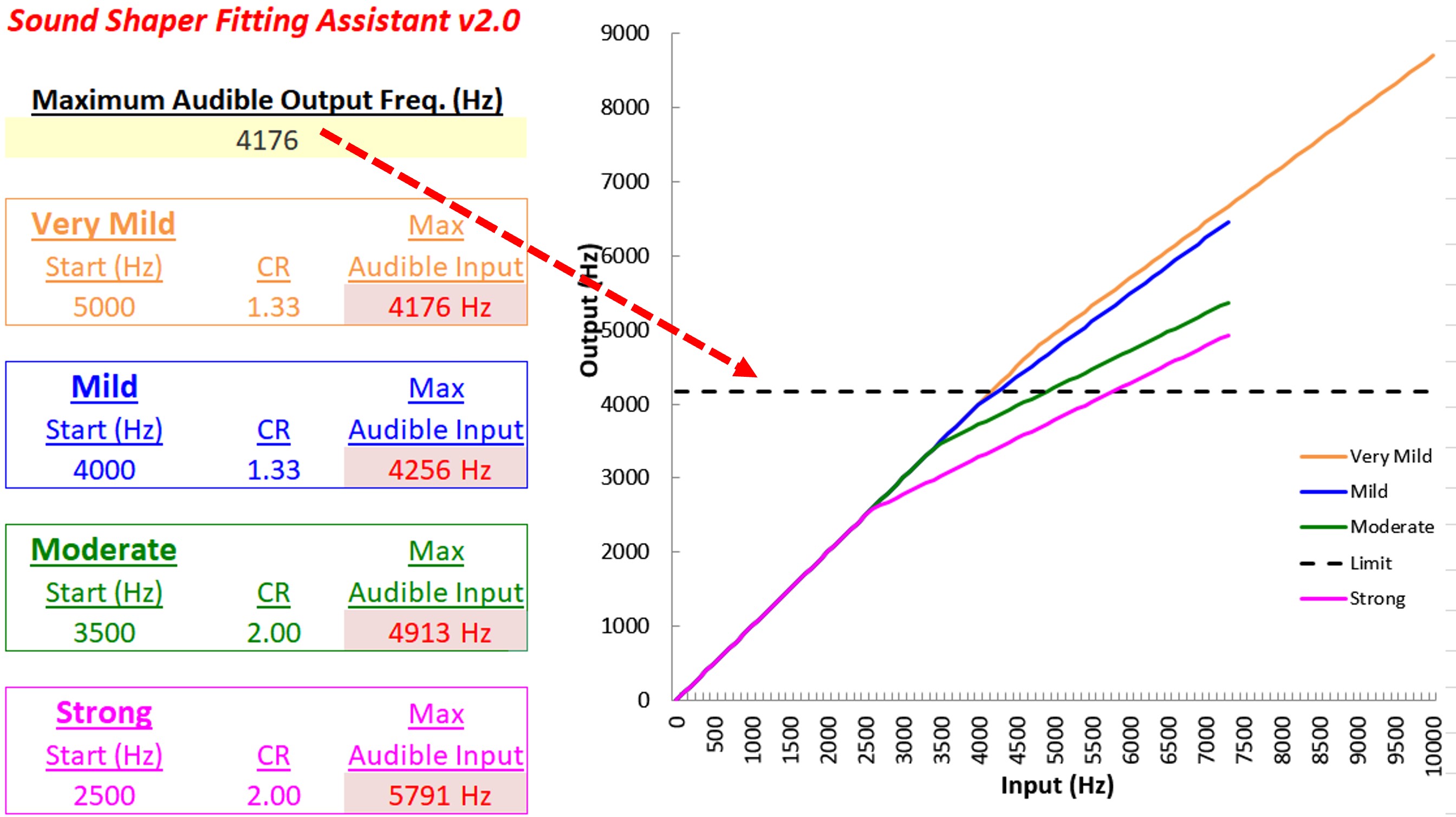
Figure 54. Screenshot of ReSound’s fitting assistant displaying three potential frequency compression settings for the first example. The only number the clinician enters is the maximum audible output frequency. Like the others, this fitting assistant displays the maximum audible input frequency and plots the input-output function for each setting.

Recall that the first example had a maximum audible output frequency of 4176 Hz. It should be clear from Figure 54, and the reported values for maximum audible input frequency that the “very mild” setting is not an option since the start frequency is greater than the maximum audible output frequency. Furthermore, very little is gained with the “mild” and “moderate” settings. Finally, the only viable option for this example is the “strong” setting, which starts at 2500 Hz and will increase the audible frequency range from 4176 Hz to 5791 Hz.

Fitting Assistant: Example 2

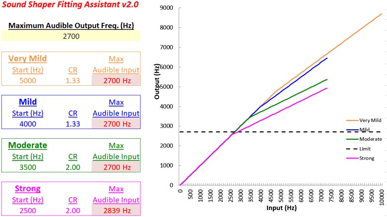
Figure 55. Screenshot of ReSound’s fitting assistant displaying three potential frequency compression settings for the second example.

Finally, with the second example, where the maximum audible output frequency was 2700 Hz, you can clearly see from Figure 55 that none of the frequency compression settings will be of use to this hearing aid user since they cannot hear any of the frequency-lowered information.

Phonak (Current) Frequency Lowering

Part X discusses the most recent method of frequency lowering, which Phonak introduced in 2016. It is a variation of their classic original nonlinear frequency compression, but its behavior is adaptive over time and depends on the incoming spectrum.

Frequency Lowering Method

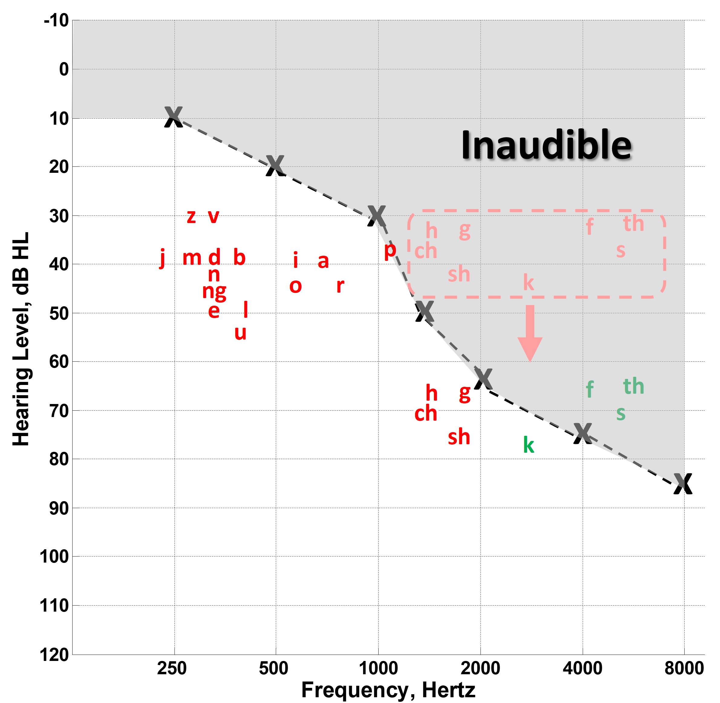
Figure 56. Illustration of the speech spectrum for high-frequency sloping hearing loss, with the gray area indicating inaudible high-frequency consonants. The red box shows the effects of hearing aid gain as demonstrated by the shift of these sounds close toward audibility for some but not all sounds.

Figure 56 depicts the speech spectrum in the same manner as Figure 3. For typical high-frequency sloping hearing losses, most of the energy of importance for high-frequency consonants is inaudible, as shown in the gray region. The primary job of hearing aids is to provide gain to make these sounds audible, as indicated by the shift of speech sounds in the red box towards higher levels (down on the graph).

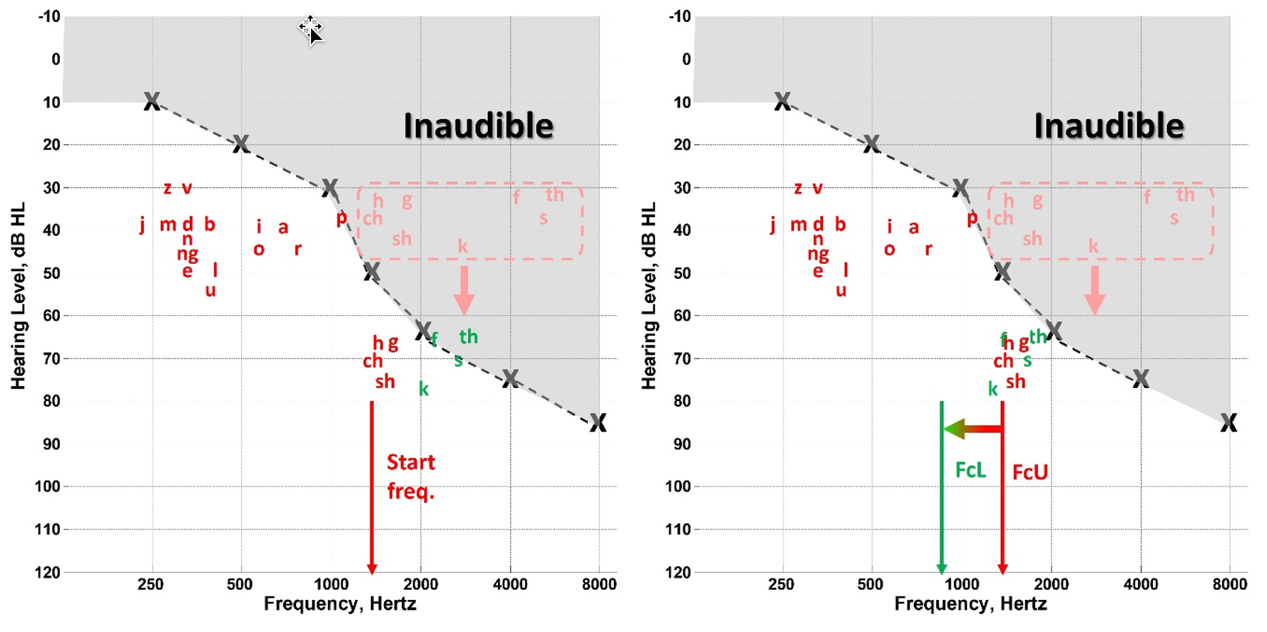
Figure 57. Left panel - Depicts traditional nonlinear frequency compression, compressing high-frequency sounds (e.g., “ch,” “sh,” “h,” “g,” “k,” “f,” “s,” “th”) towards a predetermined start frequency. Right panel - Demonstrates the adaptive aspect of the Phonak method: when higher high-frequency energy than low-frequency energy is detected in the incoming spectrum (marked in green), an additional linear frequency shift is applied, moving these sounds to an even lower frequency. In this context, the original start frequency is redefined as the upper cut-off frequency (FcU), and the extent of the additional shift is determined by the lower cut-off frequency (FcL).

As shown by left panel in Figure 57, adaptive nonlinear frequency compression begins like the old method by compressing high-frequency sounds (compare “ch,” “sh,” “h,” “g,” “k,” “f,” “s,” and “th” on Figure 56) toward a set start frequency. However, it is novel because when it detects that the incoming spectrum has greater high-frequency energy than low-frequency energy, as shown by the speech sounds in green, it undergoes an additional linear frequency shift towards an even lower frequency, as shown by the right panel of Figure 57. The start frequency (left panel) is renamed the upper cut-off frequency or FcU (right panel), while the lower bound of the linear shift is known as the lower cut-off frequency or FcL.

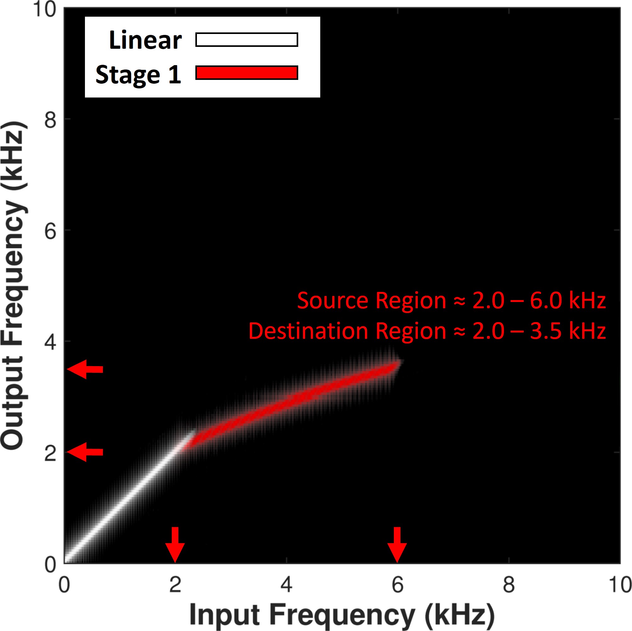
Figure 58. Spectrogram illustrating conventional nonlinear frequency compression in a hearing aid, with input frequencies on the x-axis and output frequencies on the y-axis. The white band shows frequencies below the start frequency unchanged in output, while the red band depicts compression of input frequencies from 2 to 6 kHz into an output range of 2 to 3.5 kHz.

To help illustrate what happens in the frequency domain with the new method of frequency lowering, Figure 58 shows an actual spectrogram that shows how conventional nonlinear frequency compression affects the frequencies going into the hearing aid. For a puretone sweep, the x-axis shows the input frequencies, and the y-axis shows where those frequencies go at the output. The white energy band corresponds to frequencies below the start and shows how frequencies go out at the same frequencies they went into the hearing aid. The red band shows how the source band between 2 to 6 kHz in the input goes out at the destination band between 2 to 3.5 kHz in the output.

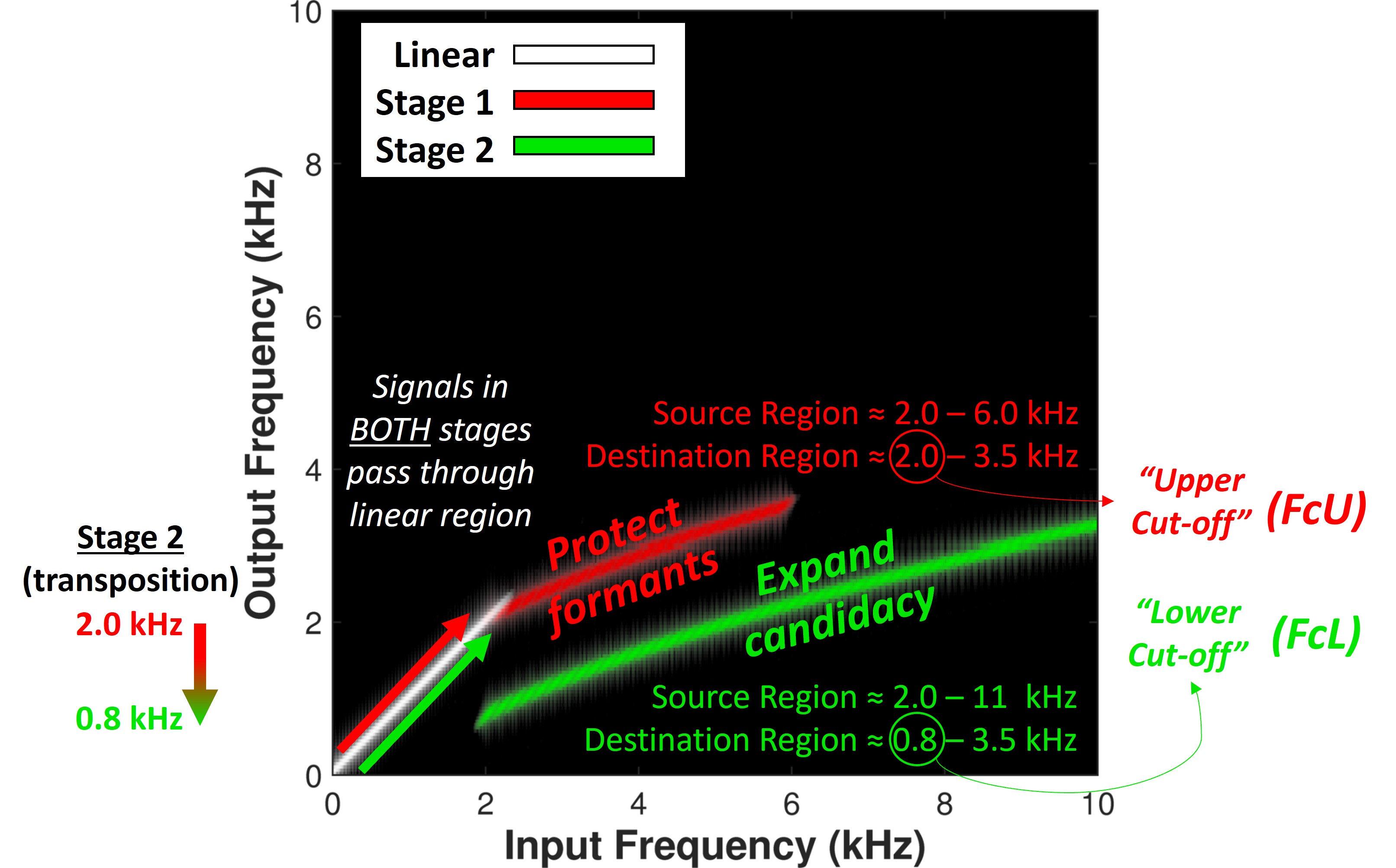
Figure 59. Demonstration of adaptive nonlinear frequency compression with a two-stage lowering process. The red energy band shows the initial stage, similar to conventional compression. The second stage, indicated by the green band, involves an additional lowering of high-frequency emphasis sounds (e.g., fricatives) by a fixed shift. This stage blends these sounds with existing lower frequencies. In this example, the 2 kHz start frequency becomes the upper cut-off for sounds with lower frequency emphasis, while a new lower cut-off for high-frequency emphasis sounds is set at 0.8 kHz. This approach allows less aggressive compression for formant-rich sounds like vowels, preserving speech clarity, while enabling a broader range of audibility, particularly beneficial for users with restricted hearing ranges.

Recall that adaptive nonlinear frequency compression starts the same way as the conventional form but then transposes high-frequency emphasis sounds in a second stage of lowering, as shown in Figure 59 by the green energy band with a fixed shift of 1.2 kHz starting at 2 kHz. It is important to note that even though frequencies are shifted below the original start frequency, they will be mixed with whatever energy is already there because sounds in both lowering stages will pass through the linear region. As discussed below, this will affect how similar or different the frication spectra for the [s] and [sh] are on the low-frequency side of the spectrum. 

As shown in Figure 59, the destination region that initially started at 2 kHz becomes the upper cut-off for low-frequency emphasis sounds, especially those dominated by formant energy, such as vowels. The new destination region for high-frequency emphasis sounds, namely frication, starts at the lower cut-off of 0.8 kHz. The rationale is that less aggressive frequency compression can be used for vowels and other low-frequency emphasis consonants to protect formants. This will help preserve speech intelligibility and sound quality. On the other hand, even lower cut-off frequencies are possible than before for frication, which serves two purposes: (1) it expands candidacy to those with a restricted range of audibility, and (2) the frequency compressed and transposed speech cues now span a wider destination range. Because less frequency compression is needed, this will help preserve the spectral detail of the original speech sound. In addition, a higher range of input frequencies can be represented in the output.

Demonstration of Algorithm Behavior

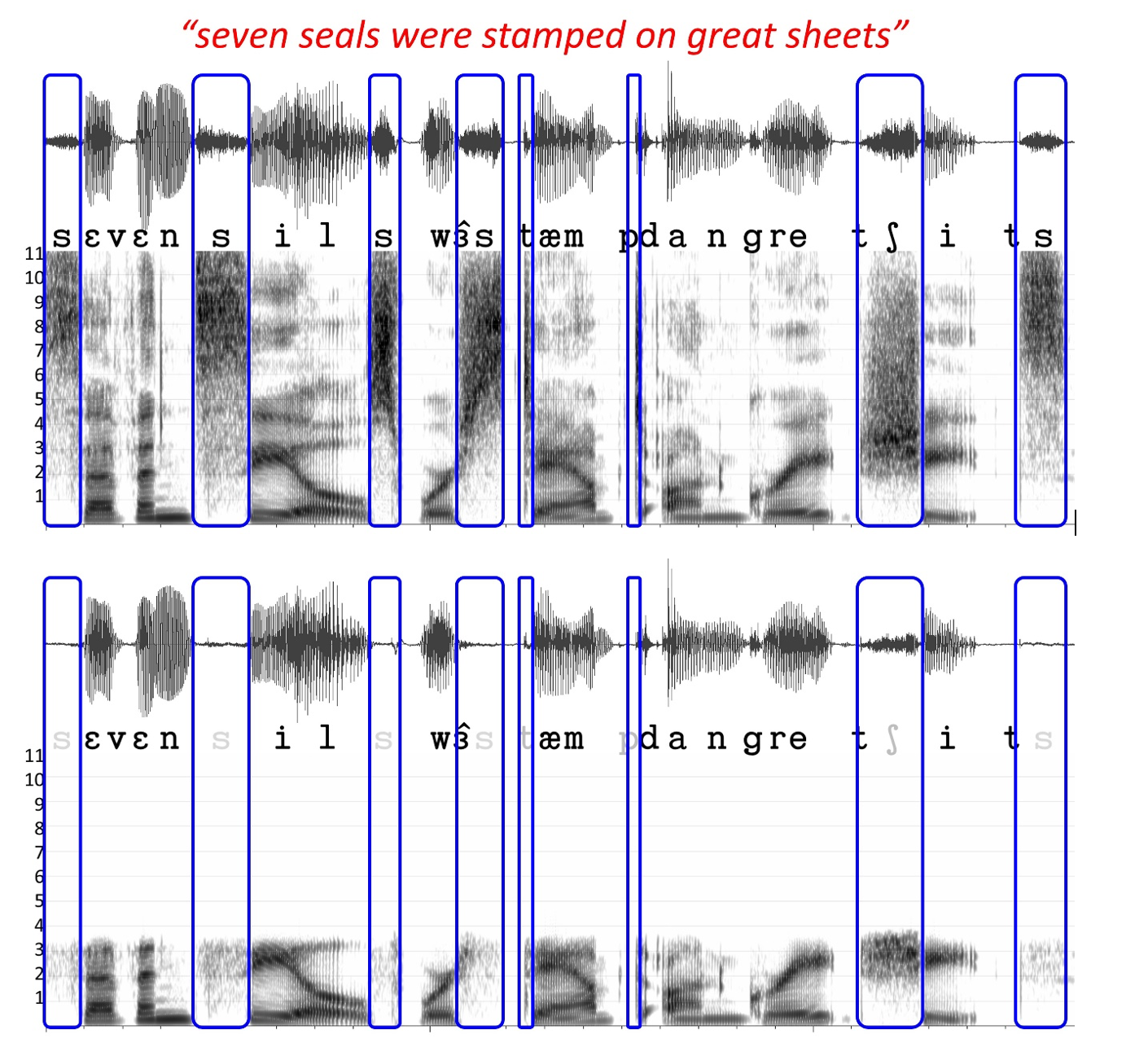
Figure 60. Spectrogram of the sentence “seven seals were stamped on great sheets,” highlighting the broad spectra of high-frequency frication in specific sounds (boxed areas) compared to the frequency-specific low-frequency formants of other sounds. Bottom - Illustration of significant high-frequency energy loss in both time waveform and spectrogram under simulated complete loss of audibility above 3.5 kHz, represented by letters in varying shades of gray.

To help see adaptive nonlinear frequency compression in action, the top of Figure 60 shows the spectrogram for the sentence “seven seals were stamped on great sheets.” Notice the contrast between the broad spectra of the high-frequency frication shown for the sounds marked by the boxes compared to the remaining sounds dominated by frequency-specific low-frequency formants. Notice the tremendous loss of high-frequency energy in both the time waveform and spectrogram at the bottom of Figure 60 when a complete loss of audibility above 3.5 kHz is simulated, as denoted by the letters in varying shades of gray.

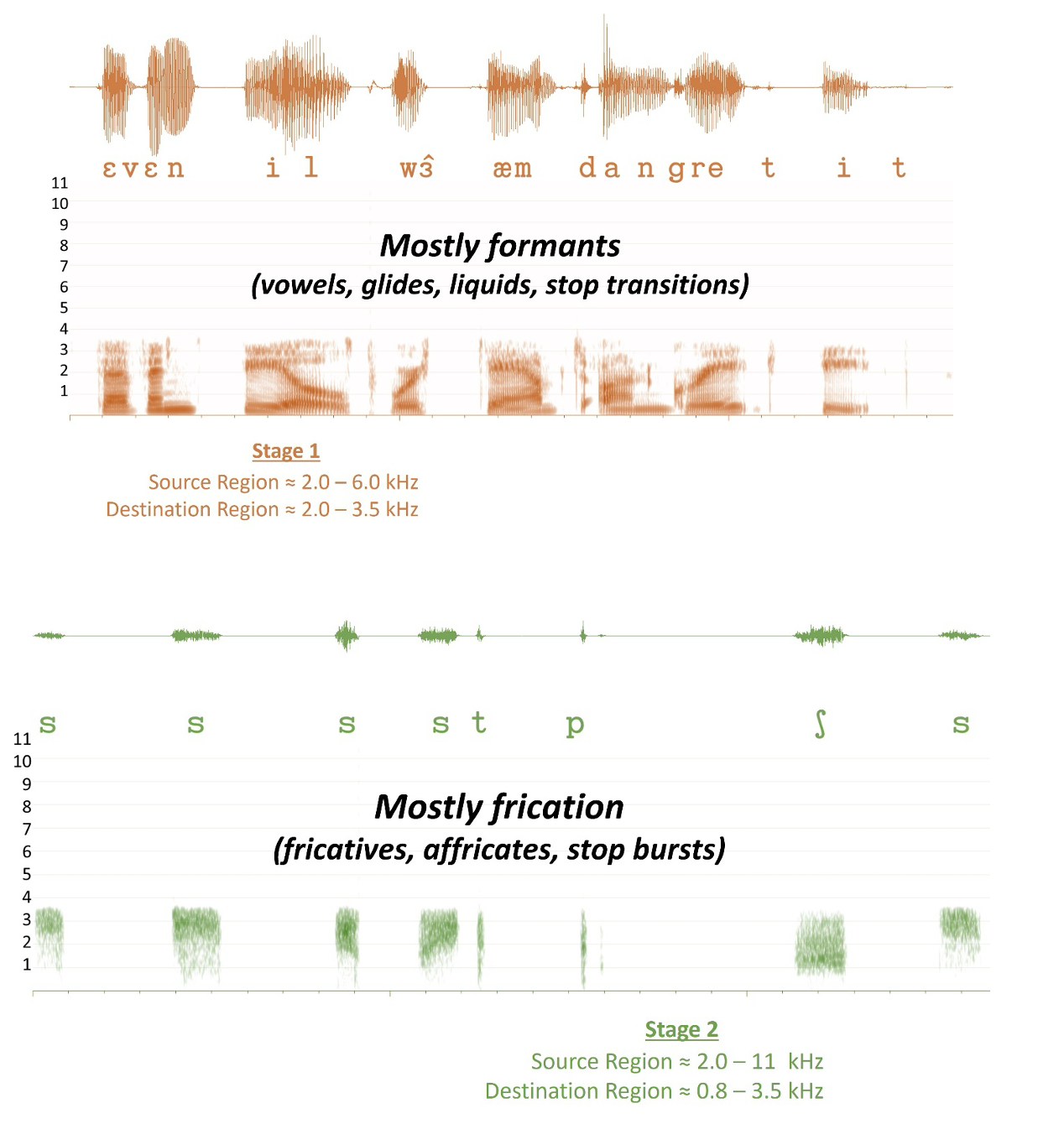
Figure 61. Demonstration of the distinct stages of adaptive nonlinear frequency compression. Top Panel: Displays speech sounds processed using only the first stage of frequency compression. This stage primarily impacts low-frequency formants found in vowels, glides, liquids, and stop consonants. Bottom Panel: Illustrates the effects of the additional transposition stage applied after compression. This stage explicitly targets high-frequency frication sounds, including the bursts from stop consonants.

Figure 61 shows what happens with each processing stage separate from the other. The top panel shows all the sounds processed with only the first processing stage. Notice that this stage exclusively affects speech sounds with low-frequency formants, like vowels, glides, liquids, and stop consonants. It is important to note that there is still frequency lowering, but it occurs over a smaller range, making it harder to see. In this example, frequency compression starts around 2 kHz, with information from 2 to 6 kHz squeezed into a range from 2 to 3.5 kHz. Again, the frequency lowering is more difficult to notice because the low-frequency formants dominate the spectrogram.

The bottom panel shows the sounds that have undergone an additional transposition after compression. Notice that this stage exclusively affects speech sounds with high-frequency frication, including the bursts of the stop consonants “t” and “p.”

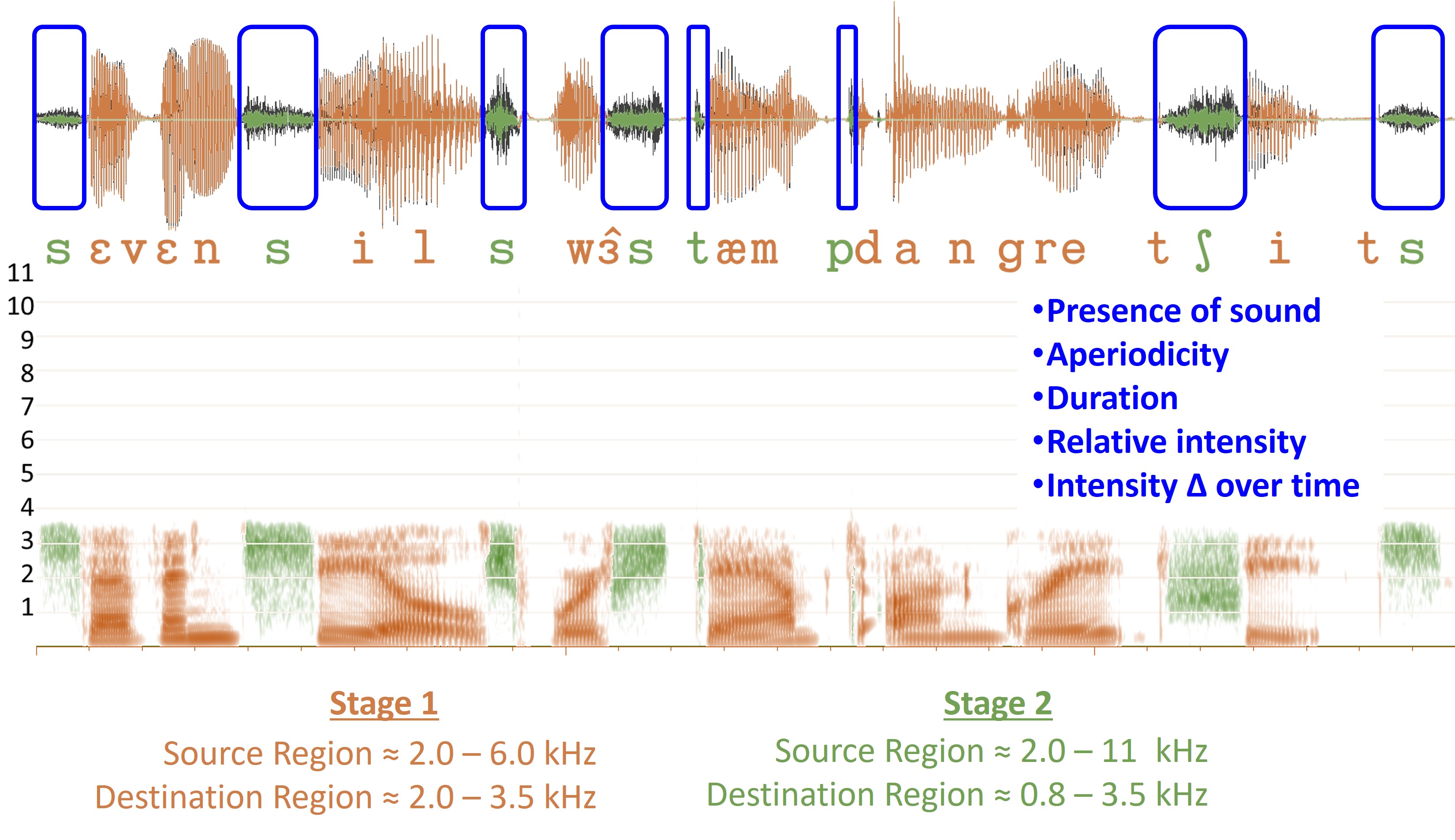
Figure 62. Combined time waveform and spectra from both stages of adaptive nonlinear frequency compression. The time waveform of the original speech, superimposed in black, highlights the similarities in the temporal envelopes, particularly in the frication sounds. This visualization underscores the key point that the frequency-lowered speech’s time waveform may contain more perceptible information than is immediately apparent from the spectrogram alone.

Figure 62 shows what the listener hears, a mixture of the two. When the time waveform of the original speech is superimposed with black, the similarities between the temporal envelopes for the frication become apparent. One of my main points is there may be more information for perception in the time waveform of the frequency-lowered speech than in the spectrogram.

Another Look at the Algorithm Behavior

To better understand the connection between the effects of the manufacturer’s programming settings on the hearing aid output and the goals of the fitting assistant, it is helpful to examine the algorithm’s behavior exclusively in the frequency domain.

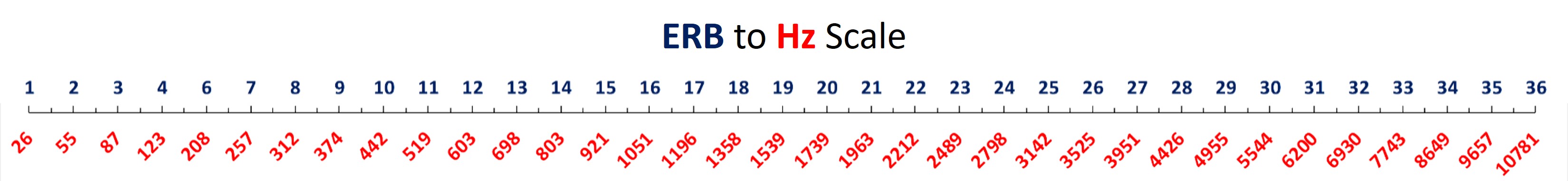
Figure 63. Graphical representation of the relationship between the Equivalent Rectangular Bandwidth (ERB) scale and Hertz (Hz), highlighting the logarithmic encoding of frequency along the cochlea.

Since the fitting assistant quantifies spectral differences between frequency-lowered [s] and [sh] sounds, as explained later, it will be important that the values have some relationship to how the auditory system encodes sounds. Therefore, I use a psychophysical scale for frequency known as the Equivalent Rectangular Bandwidth (ERB), whereby 1 ERB corresponds to one normal-hearing cochlear filter. The relationship between the ERB scale and Hz, shown in Figure 63, reflects the logarithmic nature with which frequency is encoded along the cochlea. The belief is that when the frequencies of sounds are scaled this way, the perceptual consequences will be constant along a range of frequencies.

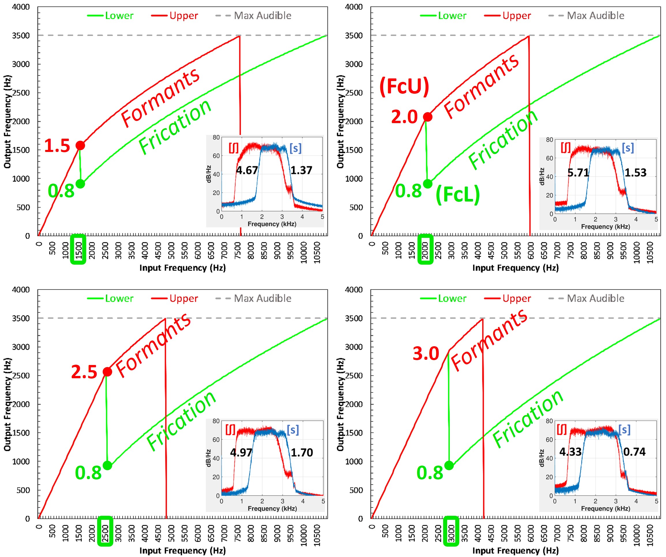
Figure 64. Illustration of the impact of the upper cut-off frequency (FcU) selection on the source region for frication in frequency lowering. Each representation in the figure maintains the same lower cut-off but varies the upper cut-off. This variation influences which frequencies are lowered along the x-axis for both the red (formants) and green (frication) input-output functions. Insets in the figure, marked in red for “sh” and blue for “s,” display their spectra, with numbers indicating the ERB differences between the edge frequencies of these sounds, offering insights into how these parameter adjustments affect auditory perception.

Figure 64 demonstrates frequency input/output functions using the fitting assistant described below. The gray dotted line shows the maximum audible output frequency at 3500 Hz. Frequencies going into the hearing aid are on the x-axis and go out at the frequencies on the y-axis. The red line is labeled “formants” since it controls low-frequency emphasis sounds, and the green line is labeled “frication” since it controls high-frequency emphasis sounds. The frequencies of sounds under control of both input-output functions are un-lowered below FcU (the upper cut-off), which is 2.0 kHz in this example. All frequencies above FcU are lowered; the only difference between the red and green functions is where the sounds go in the output.

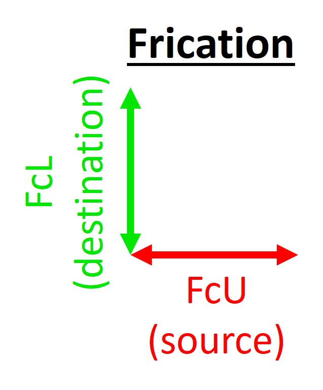
Figure 65. The lower cut-off primarily affects the output axis for frication, while the upper cut-off influences the input axis, demonstrating the interplay between these cut-offs in determining the range and extent of frequency lowering.

Here is a crucial point that may not be apparent from other descriptions of the algorithm. The source region for frication is controlled by the cut-off selected for formants. Each figure has the same lower cut-off but a different upper cut-off. Notice how the selection of upper cut-off frequency affects the frequencies that will be lowered along the x-axis for both the red and green input-output functions. From this perspective, as depicted in Figure 65, the lower cut-off operates on the output axis for frication while the upper cut-off operates on the input axis.

The advantage of doing these manipulations in a controlled fashion is that we can have precise knowledge about their effects on speech acoustics. For example, the spectra for “sh” in red and “s” in blue are shown by the Figure 64 insets. The numbers correspond to the differences in ERBs between the edge frequencies of the two sounds, allowing us to go back later and see how these changes influence perception. This exercise shows you how simple changes in just one parameter can influence the spectral shapes of the sounds leaving the hearing aid.

Programming Software Settings

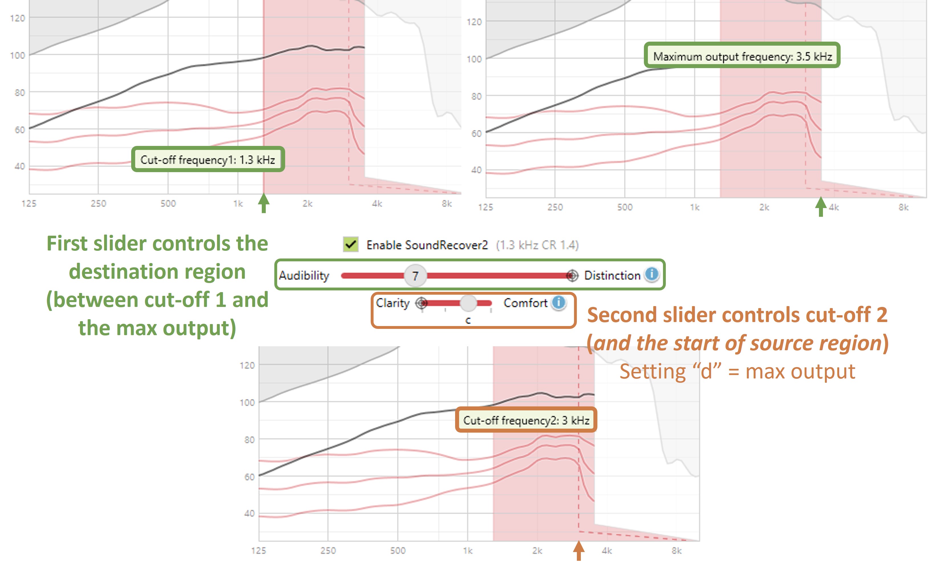
Figure 66. Displays of the programming interface of Phonak’s Target 9.0 software, featuring two adjustable settings: the audibility-distinction setting (green outline) and the comfort-clarity setting (orange outline). The audibility-distinction setting, adjustable from 1 to 20 steps on a slider, controls the destination region between the lower cut-off frequency (1.3 kHz in this example) and the maximum output frequency (3.5 kHz here). This region is where high-frequency sounds are placed post-lowering. The comfort-clarity setting, adjustable in 4 steps labeled ‘a’ to ‘d,’ dictates the upper cut-off frequency, determining the start of the source region for different sound types and preserving low-frequency formants. With 20 steps in audibility-distinction and 4 in comfort-clarity, there are 80 unique settings for each audiogram. Notably, setting ‘d’ on the comfort-clarity slider aligns the upper cut-off frequency with the maximum output frequency, deactivating frequency lowering for low-frequency sounds. Values like cut-off frequencies are not directly visible but can be seen by hovering the cursor over the relevant line in the software, which is essential for use with the fitting assistants.

As shown in Figure 66, SoundRecover2 is programmed in the software using two adjustable settings. One (outlined in green) is called the audibility-distinction setting, which is varied on a slider from steps 1 to 20. The other is called the comfort-clarity setting (outlined in orange), which is varied on a slider in 4 steps labeled ‘a,’ ‘b,’ ‘c,’ and ‘d.’ For each of the 20 settings along the audibility-distinction slider, there are 4 unique settings along the comfort-clarity slider, resulting in 80 total settings for each audiogram. Furthermore, the actual parameters assigned to each of the 20 numbers will differ depending upon the audiogram, so setting 7c shown here will correspond to a different combination of parameters than setting 7c for another audiogram.

The audibility-distinction slider controls the destination region, which is between the lower cut-off frequency (“cut-off frequency1”), as shown to be 1.3 kHz in the left panel of Figure 66, and the algorithm’s maximum output frequency, as shown to be 3.5 kHz in the right panel. Recall that the lower cut-off frequency is where the high-frequency sounds go after the second stage of frequency lowering. Be aware that the maximum output frequency is not the same as the maximum audible output frequency you determine from where the amplified speech crosses the hearing aid user’s audiogram. Instead, it simply refers to the highest frequency that will come out of the hearing aid after frequency lowering. Also, be aware that these numbers do not just appear on the visual display; you must hover your cursor over the line to see them. This is important because you need these values when working with my fitting assistants.

The comfort-clarity slider controls the upper cut-off frequency (“cut-off frequency2”), as shown in the bottom panel of Figure 66. Recall that the upper cut-off frequency determines the start of the source region for low-frequency dominated and high-frequency dominated sounds. Also, recall that to preserve the formants for low-frequency dominated sounds, it is best to set this value at 2.2 kHz or greater. Finally, note that when you put the comfort-clarity slider at setting ‘d,’ it sets the upper cut-off frequency to the same value as the maximum output frequency, effectively turning off frequency lowering for low-frequency dominated sounds.

Fitting Assistant: Goals

Using the information from “Another Look at the Algorithm Behavior,” I have developed two fitting assistants for SoundRecover2. The first version employs the principle of maximizing the non-overlap between the “s” and “sh” sounds after lowering. The goal is to maximally separate these along the cochlea in terms of the ERB scale while keeping them audible. Based on information from one of my studies, listeners need a difference of at least four cochlear filters or ERBs on the low-frequency edge to detect the two bands of noise as being different from one another. If we can reasonably separate the frequency-lowered “s” and “sh” sounds along the high-frequency side, the smallest detectable difference is 3 ERBs along each edge or 6 ERBs total. However, this is hard to do in practice with high-frequency hearing loss.

Because most of the differences between the frequency-lowered sounds will be along the low-frequency edges using the technology available today, I advise striving for a minimum difference of 5 ERBs total.

Based on one of my other studies, the second version of the fitting assistant employs the principle of minimizing the average bandwidth of the frequency-lowered “s” and “sh” sounds. It is hypothesized that this leads to better phoneme discrimination because it preserves the temporal modulation characteristics listeners can use to classify these sounds.

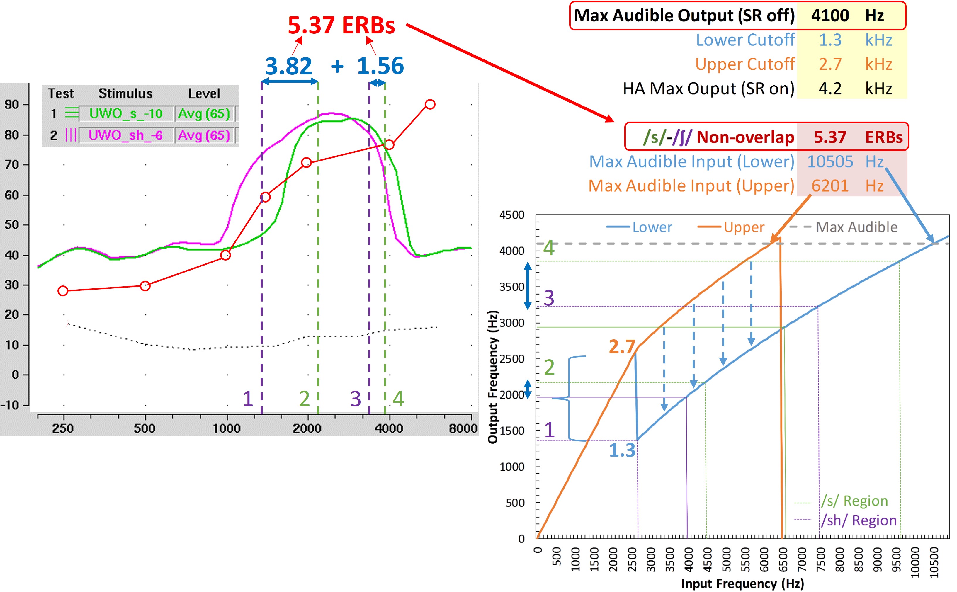
Figure 67. Screenshot of the first version of a fitting assistant designed for SoundRecover2, focusing on quantifying audible overlap between frequency-lowered "s" and "sh" sounds in terms of cochlear distance or ERBs. Right Panel: Displays two input-output functions (orange and blue lines). The orange line, with an upper cut-off at 2.7 kHz, compresses low-frequency dominated sounds, aiming to preserve low-frequency formants. The blue line, with a lower cut-off at 1.3 kHz, activates for high-frequency dominated sounds. The algorithm shifts the orange line down to the blue line’s cut-off, mixing sounds within these frequency ranges. The maximum audible output frequency, plotted as a gray dotted line (4100 Hz in this example), defines the audibility range for each signal. The maximum audible input frequencies for low-frequency (6201 Hz in this example) for high-frequency dominated sounds (10,505 Hz in this example) are displayed. Left Panel: Screenshot of the output for calibrated “s” (green) and “sh” (magenta) sounds from the Verifit for the SoundRecover2 settings. The fitting assistant matches the low and high-frequency shoulders of these sounds (purple and green lines) with their corresponding points on the Verifit output. ERB Calculation: The assistant calculates the ERB distance between the shoulders of the two sounds, summing them to gauge the total non-overlap. One recommended goal is to achieve at least a 5-ERB separation between these frequency-lowered sounds for clearer perception, with greater separation being more favorable. From this perspective, the fitting assistant provides a detailed and precise approach to optimizing SoundRecover2 settings, ensuring minimal overlap between crucial speech sounds for enhanced clarity and intelligibility.

Figure 67 shows the first version of my fitting assistant for SoundRecover2. It is designed to quantify the amount of audible overlap between the frequency-lowered “s” and “sh” sounds in terms of cochlear distance or EBRs. The right panel may appear busy with information compared to the other fitting assistants, so I will explain each component. First, we have the two input-output functions shown by the orange and blue lines. The orange input-output function has the upper cut-off and will be triggered by low-frequency dominated sounds. In this example, the upper cut-off is set at 2.7 kHz, at which point it will start compressing the spectrum. Recall that the idea is to start frequency lowering at a higher frequency to help preserve the low-frequency formats. The input-output function in blue has the lower cut-off frequency and will be triggered by high-frequency dominated sounds. In this example, are lower cut-off is set at 1.3 kHz.

Recall that functionally, the algorithm shifts the orange line down to the new cut-off frequency to create the blue input-output function, thereby mixing with the sounds concurrently present between the cut-off frequencies. In this example, the maximum audible output frequency was 4100 Hz. This value is plotted on the graph with the gray-dotted line to indicate the frequency ranges over which each lowered signal is audible. The input frequency where each input-output function crosses the gray dotted line is the maximum audible input frequency. For this example, the maximum audible input frequency for low-frequency dominated sounds is 6201 Hz and 10,505 Hz for high-frequency dominated sounds.

The left panel in Figure 67 shows the actual output of the calibrated “s” and “sh” sounds built into the Verifit for the SoundRecover2 settings in the right panel. The “s” is shown in green, and the “sh” is shown in magenta. The vertical purple line on the Verifit output with the number “1” corresponds to the low-frequency shoulder of the “sh,” which is accurately reported by the line labeled “1” in the fitting assistant. Likewise, the green lines labeled “2” on each panel correspond to the low-frequency shoulder of the “s.” Next, the purple lines labeled “3” correspond to the high-frequency shoulder of the “sh,” and the green lines labeled “4” correspond to the high-frequency shoulder of the “s.”

Finally, the fitting assistant computes the ERB distance between the shoulders of the two sounds and adds them together for the total non-overlap. Recall that the working hypothesis in this version is to strive for at least a 5-ERB separation between these frequency-lowered sounds, with more separation being better.

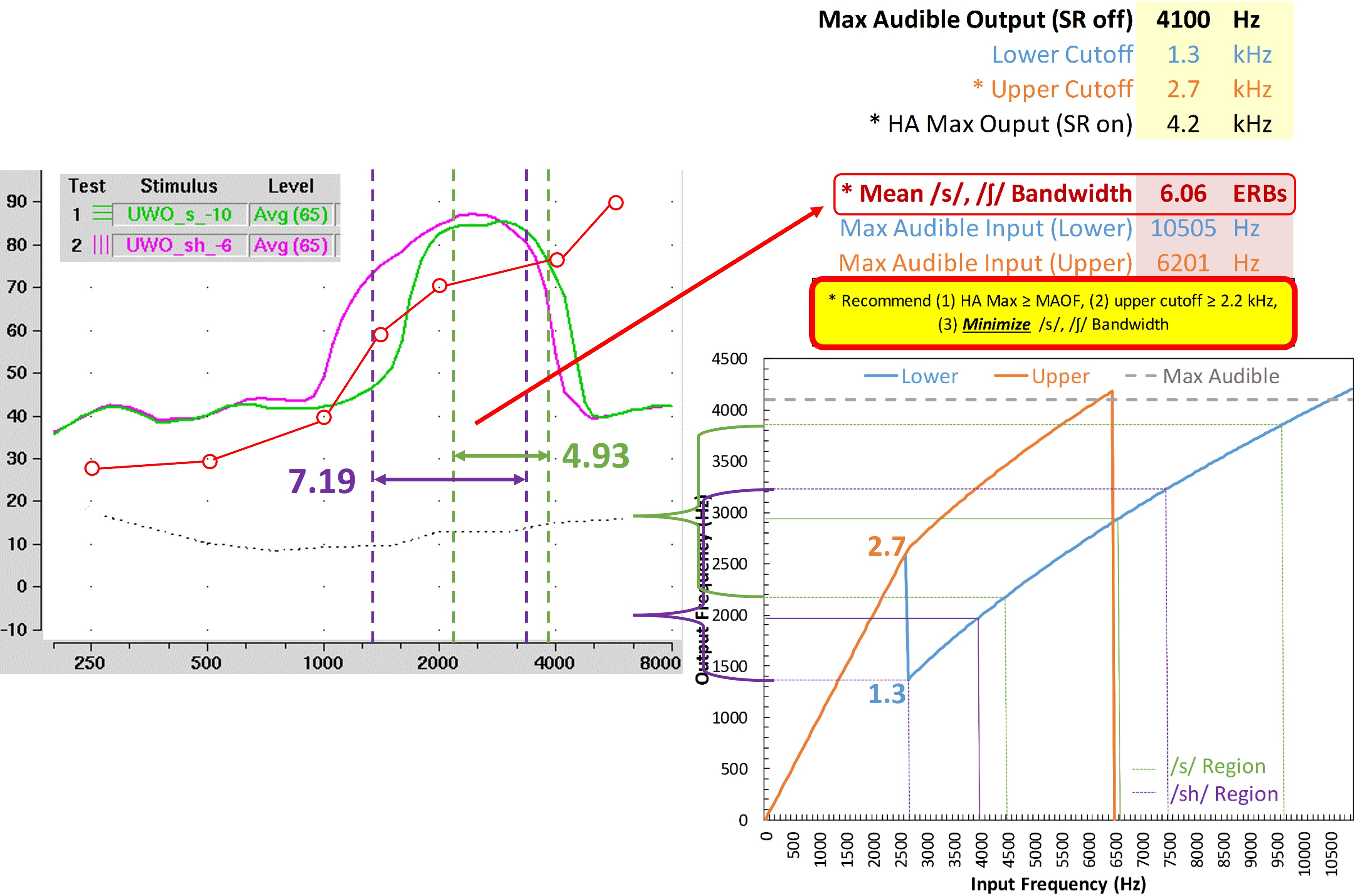
Figure 68. Screenshot of the second version of the fitting assistant, utilized in subsequent examples. The layout is similar to the first version but with a key difference in the computation approach. Bandwidth Calculation: Instead of measuring the frequency difference between the “s” and “sh” shoulders, this version calculates the bandwidth of each sound. In this example, the bandwidth for the frequency-lowered “sh” is determined to be 7.19 ERBs, while for the frequency-lowered “s,” it is 4.83 ERBs. Bandwidth Averaging: The fitting assistant averages these bandwidths, providing a single value representing the overall spectral compression of these sounds. The working hypothesis for this version focuses on minimizing the bandwidths of frequency-lowered sounds to better preserve their temporal features, enhancing their clarity and distinctness.

Figure 68 displays the second version of the fitting assistant, which I will use for the following examples. Everything appears as before; however, instead of computing the frequency difference of the corresponding shoulders between “s” and “sh,” it computes the frequency difference of the shoulders within each to derive their bandwidths. So, in this example, the frequency-lowered “sh” bandwidth is computed to be 7.19 ERBs, and the frequency-lowered “s” bandwidth is computed to be 4.83 ERBs. The bandwidths are averaged and reported by the fitting assistant. Recall that the working hypothesis in this version is to minimize the bandwidths of the frequency-lowered sounds to better preserve their temporal features.

Finally, recall that the maximum output frequency of the hearing aid, as indicated by “HA Max,” should be at least as high as the maximum audible output frequency so that the frequency lowering does not restrict the audible bandwidth for the hearing aid user. In addition, if possible, you should strive to have the upper cut-off frequency at least 2.2 kHz to better preserve the formants.

A 2-Step Approach for Working with SoundRecover2: Step 1

When working with SoundRecover2, I recommend a 2-step approach. The first step is to adjust the audibility distinction slider since it controls the maximum frequency output by the hearing aid, which they call “max output frequency.” Of the 20 available settings, you only want to consider the settings where the maximum output frequency in the programming software is greater than or equal to the maximum audible output frequency from the speechmapping; otherwise, you will reduce the audible bandwidth for the hearing aid user.

You might be tempted to set the max output frequency equal to the MAOF. However, recognize that this will mean the entire source region up to 11 kHz will be pushed down to the hearing aid user’s audible range, which might be overkill even for hearing losses with a modestly restrictive MAOF. By setting the max output frequency greater than the MAOF, you can reduce the amount of frequency compression. The tradeoff is that the highest input frequency that will be audible after lowering may only be 8, 9, or 10 kHz, for example. This is probably sufficient for hearing losses where the MAOF is only 3 or 4 kHz.

Recall that the maximum audible output frequency was 4176 Hz for the first audiogram example used throughout. First, use the audibility-distinction slider to eliminate all settings with a maximum output frequency below 4176 Hz. So, immediately, we can eliminate all the settings below 11, which has a maximum output frequency of 4.2 kHz. Moving the slider to the right to 12 sets the maximum output frequency at 4.4 kHz. According to the fitting assistant (discussed below), Setting 11 will make input sounds up to 10.8 kHz audible. However, setting 12 will make input sounds up to 10.1 kHz audible after lowering, which should be adequate for lowering the energy from “s”; therefore, I chose setting 12.

A 2-Step Approach for Working with SoundRecover2: Step 2

Once you have narrowed down the settings for the audibility-distinction slider to one or two options, the second step is to choose among the 4 options for the clarity-comfort slider. You may want to use one of the two fitting assistants for this. Recall that this setting controls the upper cut-off frequency, which determines the lower limit of the source regions for both low-frequency and high-frequency dominated sounds. Also, recall that setting ‘d’ effectively turns off frequency lowering for the low-frequency dominated sounds.

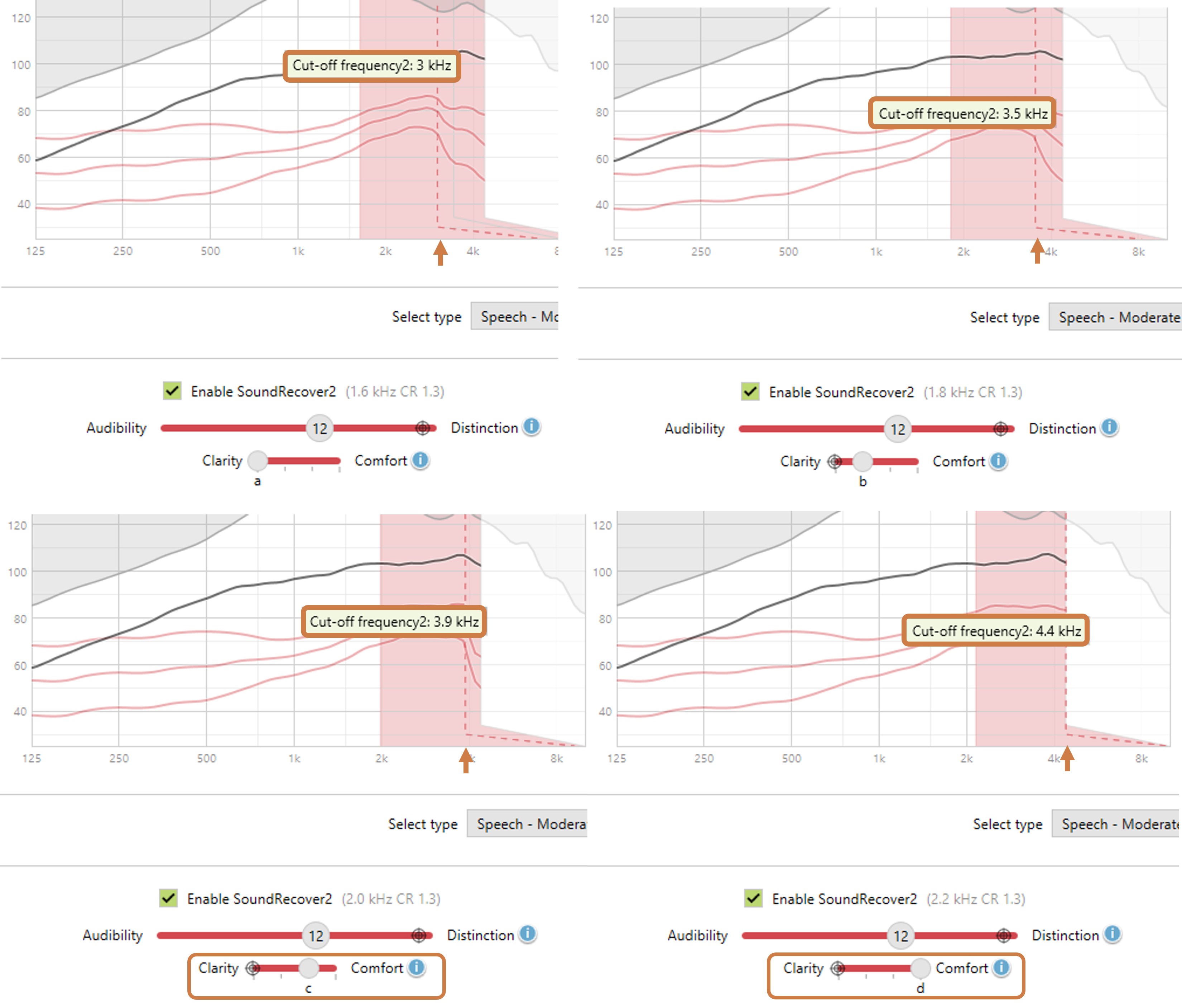
Figure 69. Process for selecting among the four comfort-clarity slider options in SoundRecover2, with the audibility-distinction setting fixed at 12 in this example. The selection involves hovering the cursor over the "cut-frequency2" line for each setting and noting the values for use with the fitting assistant. The upper-left panel displays the upper cut-off for setting 'a' as 3 kHz and subsequent panels display the upper cut-offs for the other settings. Notably, since the maximum output frequency is also 4.4 kHz, setting 'd' effectively turns off frequency lowering for low-frequency dominated sounds, preserving their natural frequencies.

Keeping the audibility-distinction setting fixed at 12, the second step is to choose among the 4 options for the comfort-clarity slider, as shown in Figure 69. You do this by hovering your cursor over the line corresponding to the “cut-frequency2” for each of the 4 settings. Write these values down since you need them when using the fitting assistant. The upper-left panel shows the upper cut-off for setting ‘a’ is 3 kHz. From top to bottom, left to right, the upper cut-off for setting ‘b’ is 3.5 kHz, 3.9 kHz for ‘c,’ and 4.4 kHz for ‘d.’ Recall that the maximum output frequency is also 4.4 kHz, so setting ‘d’ effectively deactivates frequency lowering for low-frequency dominated sounds.

Fitting Assistant: Example 1

You can use either of the two fitting assistants to help you decide which of the 4 settings for the comfort-clarity slider to select. For these examples, the second version of the SoundRecover2 Fitting Assistant is used for the reasons mentioned above.

Figure 70. Screenshot of the SoundRecover2 Fitting Assistant for setting 12a, used for the audiogram example. Key steps include entering the maximum audible output frequency from speechmapping, programming software values for Lower and Upper Cutoffs, and HA Max Output. The fitting assistant visualizes the input/output frequency ranges for “s” (green lines) and “sh” (purple lines), with the goal of minimizing their combined bandwidth, calculated here to be 5.83 ERBs.

Figure 70 shows a screenshot of the fitting assistant for setting 12a for the audiogram used to generate the first example. First, enter the maximum audible output frequency from the speechmapping when frequency lowering was turned off. Then, enter the values from the programming software. The Lower Cutoff is ‘cut-off frequency1,’ Upper Cutoff is ‘cut-off frequency2,’ and HA Max Output (SR on) is the maximum output frequency displayed in the programming software.

Recall the dotted green lines show in the input and output frequency range for the “s” sound, with the solid green line corresponding to the peak frequency for “s.” Similarly, the purple lines show the same information for the “sh” sound. Finally, recall that the goal of the second version of the SoundRecover2 Fitting Assistant is to minimize the bandwidths of the two sounds, which was computed to be 5.83 ERBs for this setting.

For reference, the goal of the first version of the SoundRecover2 Fitting Assistant is to maximize the non-overlap between these sounds. In case you are curious, this first setting had the greatest amount of non-overlap between the frequency-lowered “s” and “sh” sounds. Each successive setting that I will show resulted in more and more overlap.

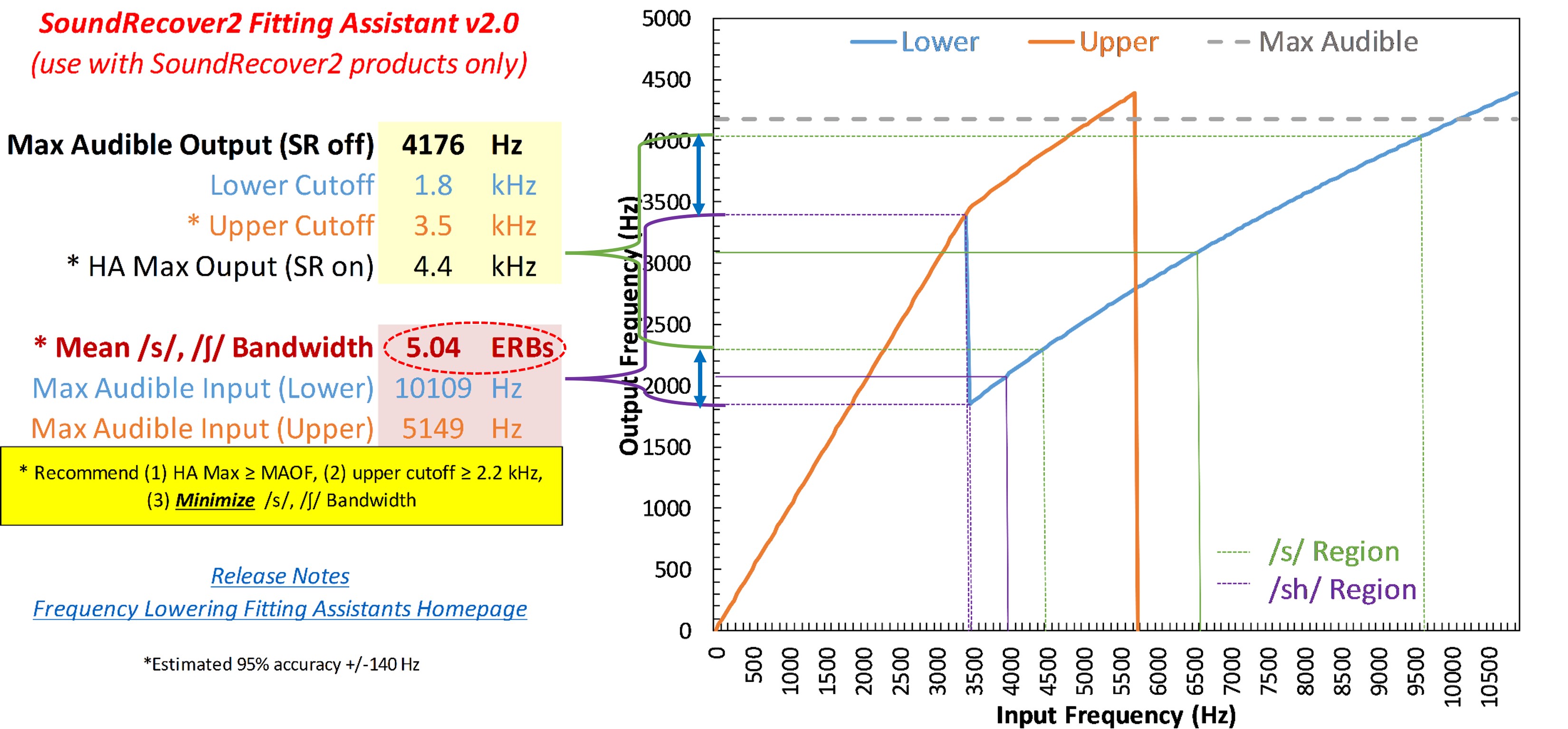
Figure 71. Similar to Figure 70 but using the 'b' comfort-clarity setting. This setting was ultimately selected as it resulted in the smallest combined bandwidths for the “s” and “sh” sounds.

Figure 71 shows the fitting assistant results when the comfort-clarity setting is ‘b.’ Ultimately, this was the chosen setting since it led to the smallest bandwidths for the “s” and “sh” sounds.

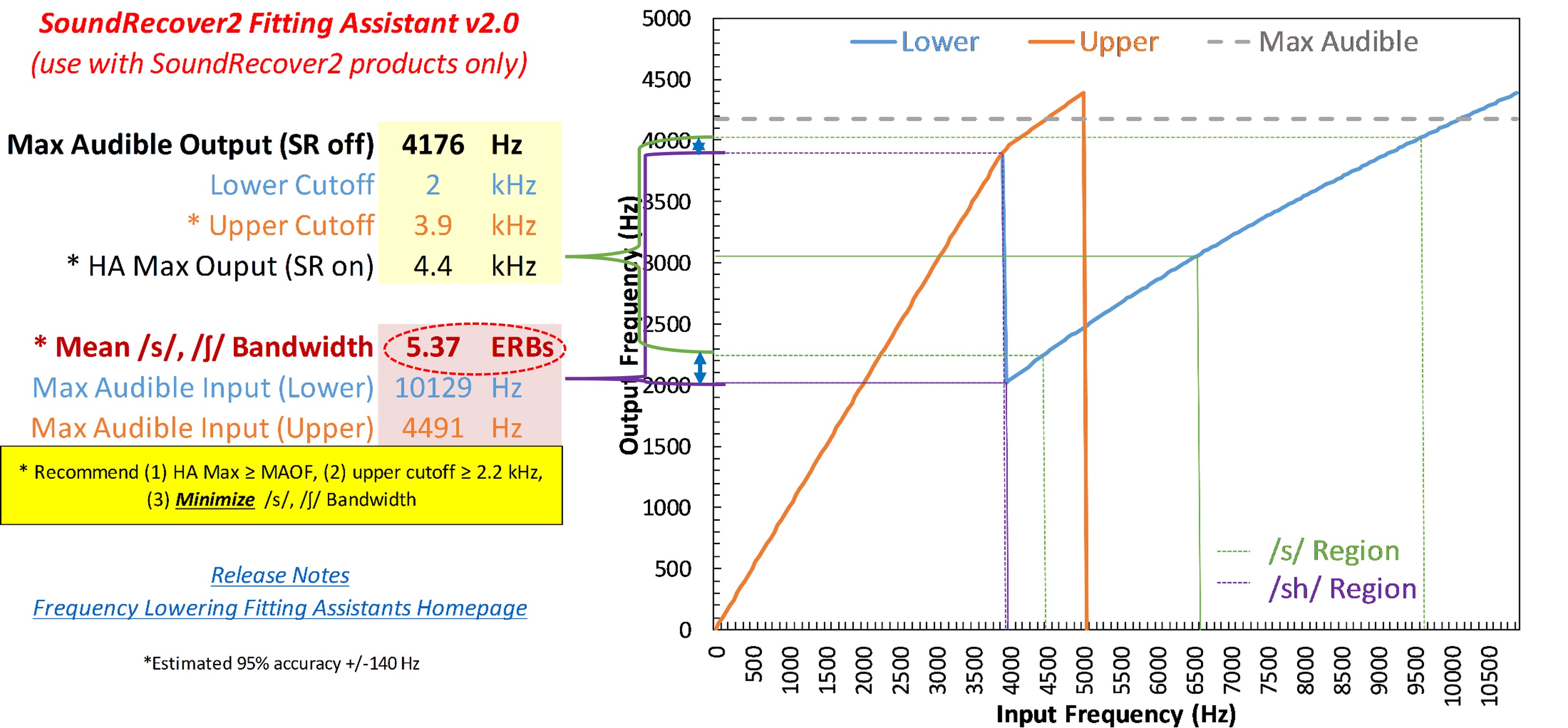
Figure 72. Similar to Figure 70 but using the 'c' comfort-clarity setting.

Compared to the first setting, 12a, setting 12c (Figure 72) results in smaller bandwidths for “s” and “sh” but more overlap. According to my data, this setting should result in better outcomes compared to 12a.

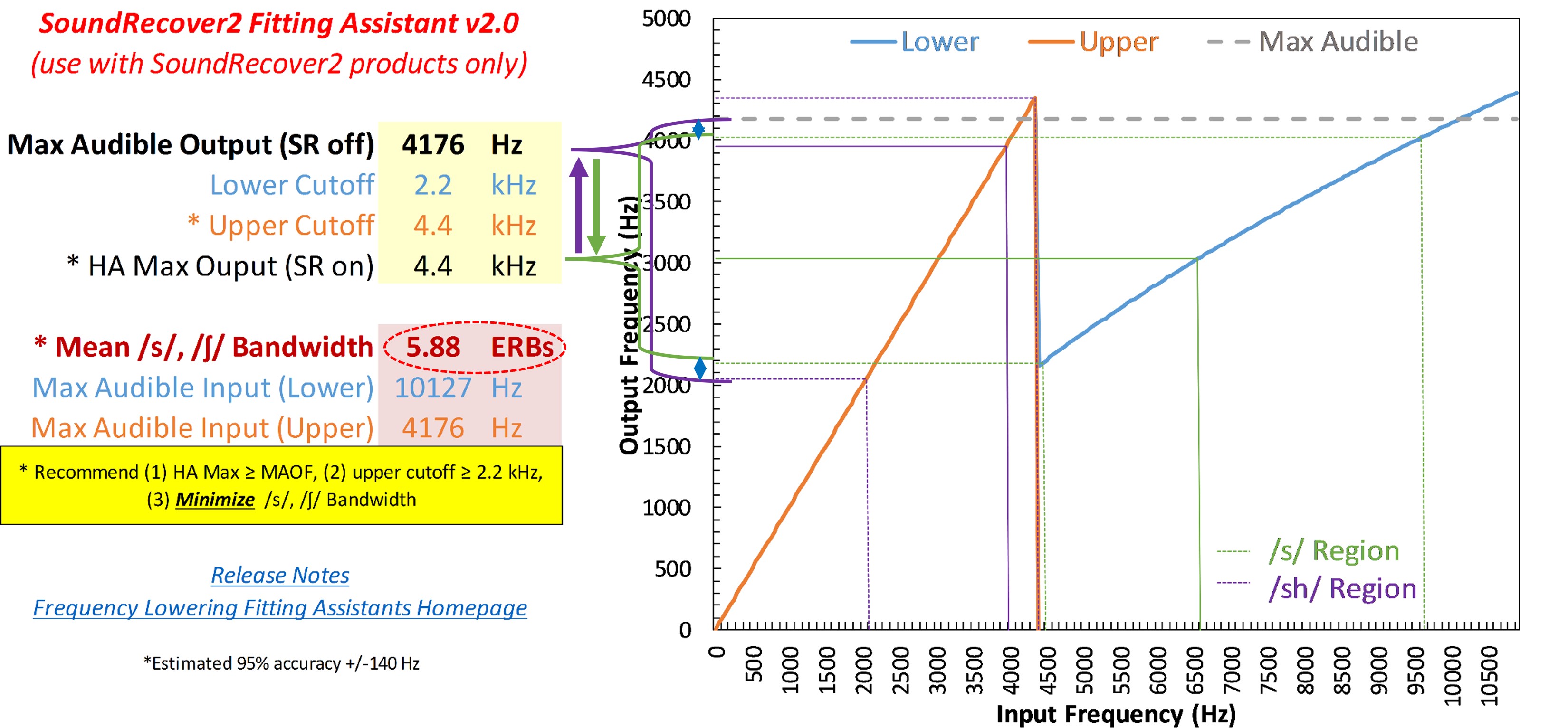
Figure 73. Similar to Figure 70 but using the 'd' comfort-clarity setting.

Finally, setting 12d (Figure 73) presents an interesting situation. First, according to both versions of the fitting assistants, it should lead to the worst outcomes because it results in the widest bandwidths for “s” and “sh” and the most overlap. Second, we see a reversal in the output frequencies for their peaks, with the peak frequency of “s” now being lower than the peak frequency of “sh”.

Fitting Assistant: Example 2

For the second audiogram example, recall that the maximum audible output frequency without frequency lowering was 2700 Hz. Again, the first step is to decide on the setting for the audibility-distinction slider. Setting 1 puts the maximum output frequency at 2.7 kHz, meaning that information up to 11 kHz would be audible to the hearing aid user after lowering, which, as I indicated earlier, is extreme overkill. Setting 2 puts the maximum output frequency at 2.8 kHz, settings 3 and 4 at 3 kHz, and setting 5 at 3.2 kHz. According to the fitting assistant, the maximum input frequencies corresponding to these maximum output frequencies are 10,882 Hz for setting 1, 10,241 Hz for setting 2, 9151-9246 Hz for settings 3 and 4, and 8304 Hz for setting 5.

I explored the fitting assistant results for both settings 3 and 4 since the maximum audible output frequencies seemed to be a good compromise between too much compression and too little high-frequency information. One could also make a strong case that setting 5 could be chosen since a maximum audible out frequency of 8300 Hz is a significant improvement over the 2700 Hz that the hearing aid user had without frequency lowering.

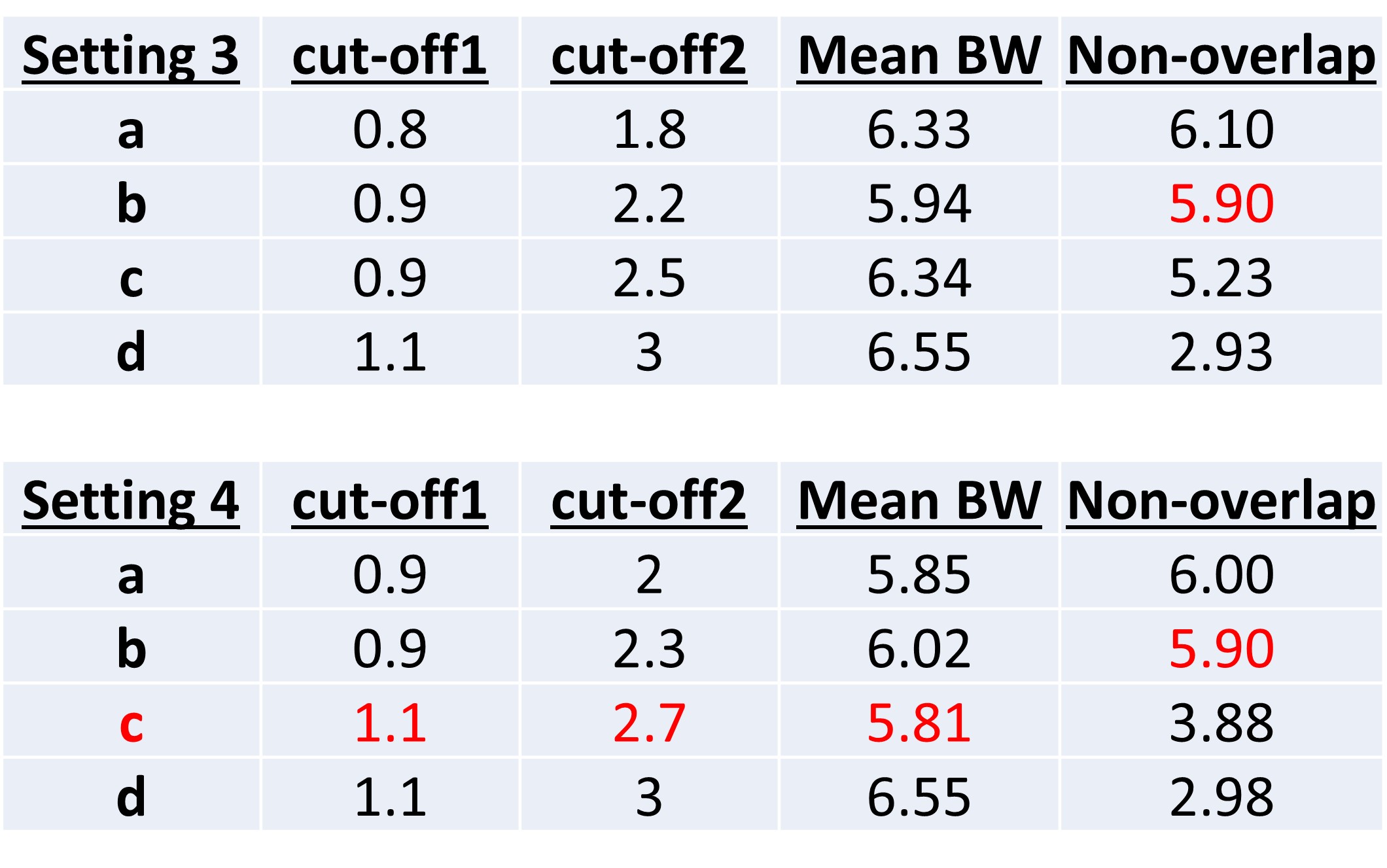
Table IV. Values for the comfort-clarity settings of SoundRecover2 when the audibility-distinction slider is set to positions 3 and 4 for the second audiogram example. Among the eight possible combinations, setting 4C emerges as the most effective, as it minimizes the average bandwidth for the “s” and “sh” sounds.

The values for the comfort-clarity settings when the audibility-distinction slider was put at setting 3 and setting 4 are shown in Table IV. As indicated, of the 8 combinations of settings, 4C minimizes the average bandwidth of the “s” and “sh.” Furthermore, remember that you want to try to keep the upper cut-off at or above 2.2 kHz to help preserve the formants of the low-frequency dominated sounds. So, setting 3a and 4a might be ruled out on this basis alone.

In case you are curious, just as before, the amount of overlap between these sounds increased as the comfort-clarity setting was successively increased from ‘a’ to ‘d,’ and the overlap was about the same for both settings of the audibility-distinction slider. Setting ‘a’ and ‘b’ had similar amounts of overlap. I would choose settings 3b or 4b because they have upper cut-off frequencies equal to or greater than 2.2 kHz.

Summary

Frequency-lowering technology in hearing aids marks a significant advancement for those with high-frequency hearing loss. It modifies sounds outside a person’s hearing range, especially high frequencies, transforming them into audible lower frequencies. This is particularly beneficial as high-frequency sounds often include critical consonants in speech, crucial for understanding spoken language. Manufacturers implement frequency-lowering in various ways, aiming to enhance speech comprehension without sacrificing the natural sound quality, thus aiding communication for individuals with hearing loss.

Frequency-lowering techniques in hearing aids, such as frequency compression and transposition, are fundamental methods used by various manufacturers to assist individuals with high-frequency hearing loss. Frequency compression works by squeezing high-frequency sounds into a lower frequency range, while frequency transposition shifts these sounds to lower frequencies without compression. These methods differ in how they process and deliver sound, each with its unique impact on speech perception and sound quality.

The impact of frequency-lowering on speech perception is a critical aspect of using this technology in hearing aids. It specifically affects the perception of high-frequency speech sounds, which are crucial for understanding speech. However, this alteration must be carefully balanced to ensure that low-frequency speech remains natural and intelligible. The effectiveness of these techniques can vary based on the individual’s audiogram and the method of frequency-lowering used.

Frequency-lowering in hearing aids comes with significant challenges and limitations. One of the primary challenges is maintaining speech clarity; altering the low frequencies can sometimes distort the natural distinctions between speech sounds that rely heavily on formants and other frequency-specific cues. Additionally, these techniques can have other potential side effects, such as unnatural sound quality, which might affect the user’s listening experience. Manufacturer recommendations also face limitations in tailoring these adjustments to individual audiograms, which is crucial for effective speech perception. These challenges underscore the need for ongoing development and refinement in frequency-lowering technology and clinical recommendations concerning individualized parameter adjustments.

In the realm of clinical practice and research, frequency-lowering presents significant barriers. Clinically, there is a gap in effectively customizing these technologies to individual audiograms, often leading to sub-optimal outcomes. Research-wise, there is a need for more in-depth studies to understand the long-term impacts of frequency-lowering on speech perception and cognitive load. These barriers highlight the necessity for enhanced research and clinical trials, aiming for a deeper understanding and better implementation of frequency-lowering technologies in hearing aids.

Different hearing aid manufacturers implement frequency-lowering technology in unique ways. Some use frequency compression, others frequency transposition, and others a pseudo-hybrid of both. Key differences between the various methods can significantly impact the effectiveness and user satisfaction with the hearing aid. This diversity in methods underscores the complexity and customization required in treating high-frequency hearing loss.

Customizing frequency-lowering in hearing aids is essential for maximizing its benefits. Personalization is critical as hearing loss varies among individuals. Customization ensures that the technology aligns with the specific audiogram of the user, thereby enhancing speech clarity and overall hearing experience. Without individualized settings, the effectiveness of frequency-lowering can be significantly reduced, as generic settings may not adequately address the unique needs of each user. This emphasis on individualization highlights the complexity and necessity of tailoring hearing aids to each user.

The future of frequency-lowering technology in hearing aids offers several promising research and development avenues. This includes refining the algorithms for more accurate and individualized frequency adjustments, enhancing the integration of these technologies into various hearing aid designs, and conducting extensive clinical trials to better understand long-term impacts on speech perception and cognitive processing. Collaborative research involving audiologists, engineers, and end-users is crucial to ensure advancements are technologically sound and practically beneficial for those with hearing impairments. Such an approach will significantly enhance the application and effectiveness of frequency-lowering technologies.